Mitch Richling: Rössler Attractor
| Author: | Mitch Richling |
| Updated: | 2021-08-02 |
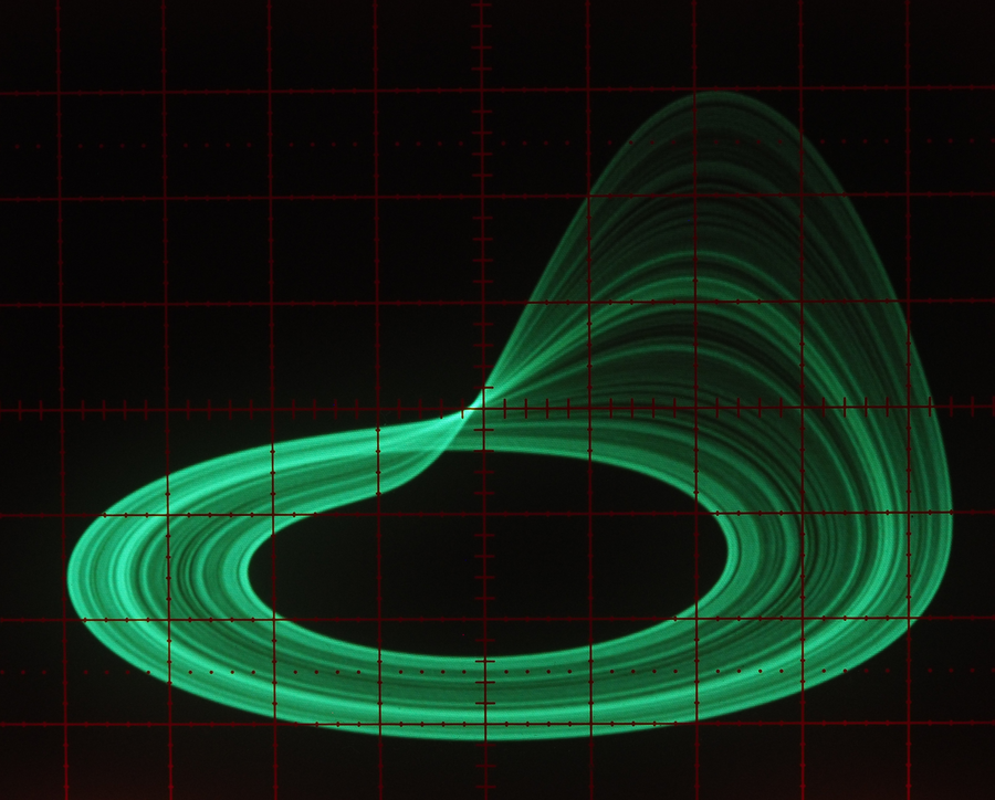
Table of Contents
1. Introduction
The Rössler attractor is a simple system of three non-linear ordinary differential equations:
\[\frac{df}{dt}=[-y-z,x+ay,b+z(x-c)]\]
Several parameter sets are commonly used:
- \(a=0.2, b=0.2, c=5.7\)
- \(a=0.18, b=0.2, c=5.7\)
- \(a=0.1, b=0.1, c=14\)
In what follows I'll be using \(b=0.4\), \(a\approx0.2\), and various values of \(c\).
2. Simulation & Visualization: Analog Computer
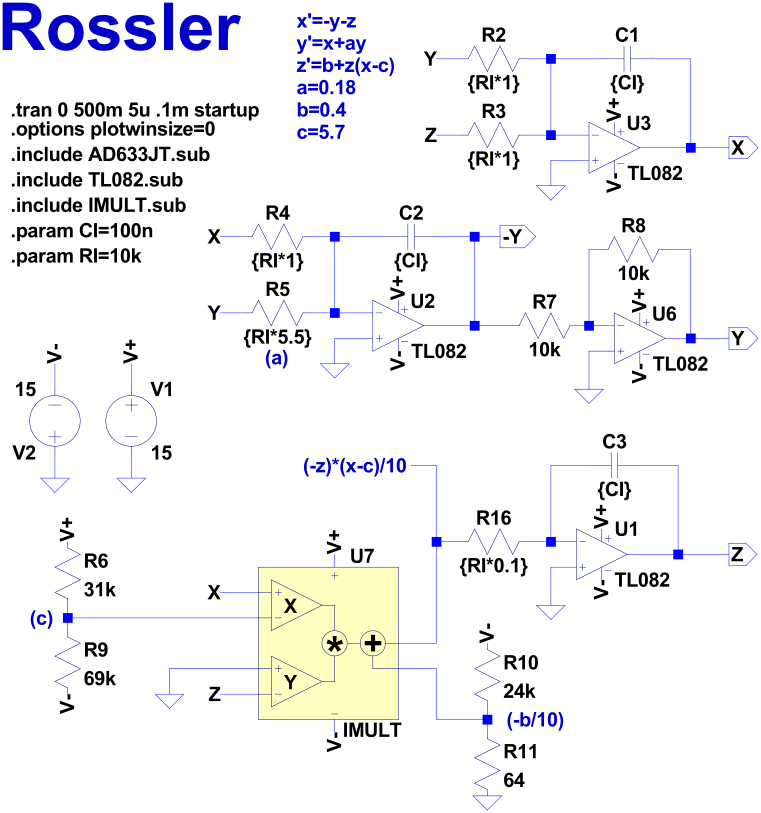
2.1. Circuit
Given any system of differential equations it is possible to find an electronic circuit governed by the same equations. These circuits are called "analogs" of the system of equations, and that's why we use the word "analog" for most non-digital electronics today. The circuit below is an analog of the Rössler system. I say an analog because many different analogs of the system exist.
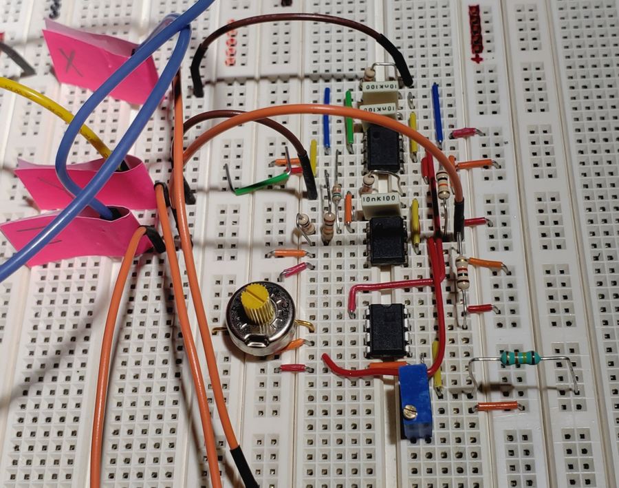
When I put this together my parts bin contained: A big bag of \(10\mathrm{K}\) resistors, a box of precision \(24\mathrm{K}\) resistors I rescued from the
dumpster at work, a bag of \(100\mathrm{nF}\) caps, and a few 10 turn \(100\Omega\) pots. Obviously many of the choices in the circuit below are more about the
parts I had on hand than anything else. ;) The resistor pair for the \(c\) coefficient are part of a single \(100\mathrm{K}\Omega\) pot. The \(64\Omega\)
resistor hanging off the multiplier is a pot. The power is important for this circuit – it must be stable and \(\pm 15\mathrm{V}\).
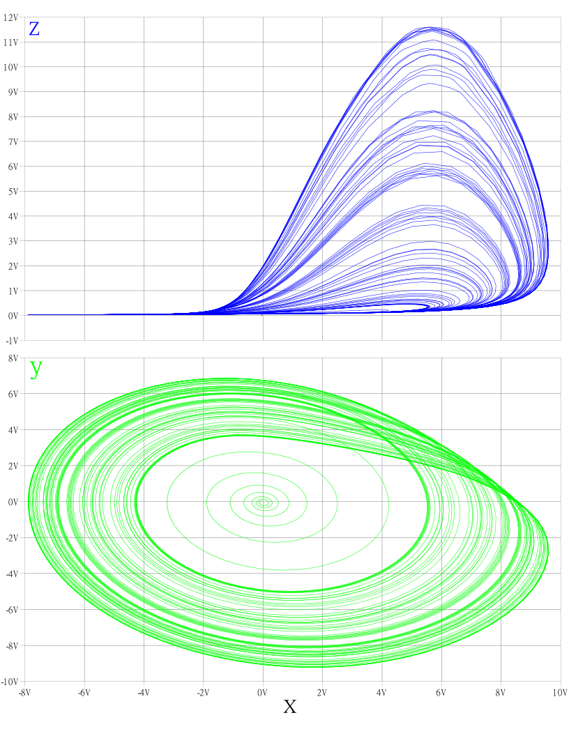
2.2. SPICE Simulation Results
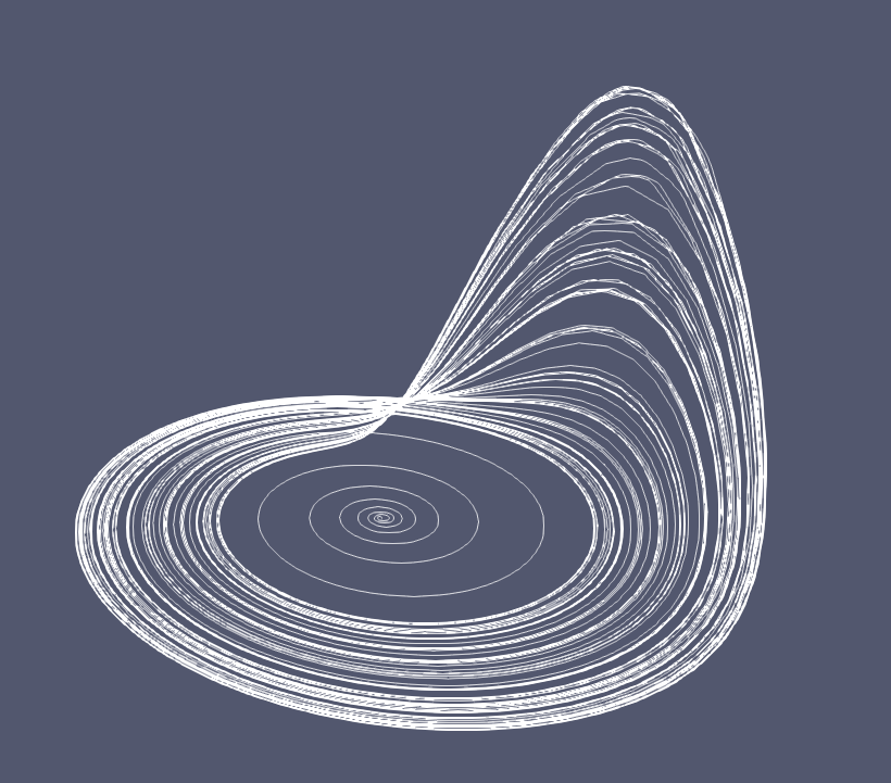
2.3. SPICE Simulation 3D Visualization
We can load the data from the spice simulation into Paraview, and interactively look at the object in 3D. Here is a screen shot:
2.4. Physical Implementation
2.5. Behavior of Physical Circuit
Note the output of the circuit is passed through another analog processing unit that translates, scales, and rotates the results – that's why the image is spinning. Someday I'll do a little write-up of that circuit…
- Scope
- Tektronix AN/USM488 (military version of the 2235). Equipped with the clear plexiglass CRT filter minus the wire mesh.
- Capture Device
- Olympus OM-D E-M1 MARK II with Olympus M.Zuiko ED 60mm f/2.8 Macro Lens
3. Failures
3.1. Close but with unwanted oscillations
- Scope
- Tektronix AN/USM488 (military version of the 2235). Equipped with the standard military wire mesh & clear plexiglass CRT filter
- Capture Device
- Olympus OM-D E-M1 MARK II with Olympus M.Zuiko ED 60mm f/2.8 Macro Lens
3.2. Interesting system near the Rossler Attractor
This is from the same circuit, but with different pot settings. The attractor is very stable.
- Scope
- Siglent Technologies SDS2504X Plus
- Capture Device
- Captured directly from scope's VNC server
3.3. Another system near the Rossler Attractor
This one is is the result of a bad connection. I like it.
- Scope
- Tektronix AN/USM488 (military version of the 2235). Equipped with the standard clear plexiglass CRT filter
- Capture Device
- Olympus OM-D E-M1 MARK II with Olympus M.Zuiko ED 60mm f/2.8 Macro Lens
4. References
Check out the chaos in electronics section of my reading list. For more about chaos in general, take a look at the fractals section of my reading list.