Mitch Richling: Measuring Impedance
| Author: | Mitch Richling |
| Updated: | 2023-03-12 |
Limited budgets mean many electronics hobbyists need to measure capacitance or inductance without an LCR meter. The method documented here adapts easily to different equipment you may have on hand – from an old fashioned audio signal generator with an analog VOM to a fancy AWG with digital oscilloscope.
Table of Contents
1. Test Circuit & Formulas
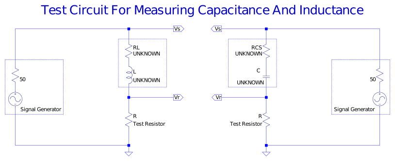
If one knows the series resistance (\(R_L\) or \(R_{CS}\)), then one may directly compute the value of \(C\) or \(L\) from \(V_R\), \(V_S\), and \(f\):
\[ C = \frac{V_{R}}{2 \pi f \, \sqrt{R^{2} V_{S}^{2} - \left(R +R_{\mathit{CS}} \right)^{2} V_{R}^{2} }} \;\;\;\;\;\;\;\;\;\;\;\;\; L = \frac{\sqrt{R^{2} V_{S}^{2} - \left(R +R_{L} \right)^{2} V_{R}^{2}}}{2 \pi f V_{R}} \]
If the series resistance (\(R_L\) or \(R_{CS}\)) may be safely ignored, then the above equations may be replaced by less complex alternatives.
\[ C = \frac{V_R}{2 \pi f R \sqrt{V_S^2-V_R^2}} = \frac{\sqrt{V_S^2-V_C^2}}{2 \pi f R V_C} = \frac{V_R}{2 \pi f R V_C} \;\;\;\;\;\;\;\;\;\;\;\;\; L = \frac{R \sqrt{V_S^2-V_R^2}}{2 \pi f V_R} = \frac{R V_L}{2 \pi f \sqrt{V_S^2-V_L^2}} = \frac{R V_L}{2 \pi f V_R} \]
Back in the day, when signal sources were higher voltage and sliderules were king, the advice was to set the generator output voltage and frequency so that \(V_S=10\mathrm{V}\) and \(V_R=1\mathrm{V}\). In this case the above simplify to:
\[ C \approx 0.01599567362 \frac{1}{f R} \;\;\;\;\;\;\;\;\;\;\;\;\; L \approx 1.583571689 \frac{R}{f} \]
Note it is the ratio \(V_S\) to \(V_R\) that really matters in the formula above (i.e. so long as \(V_S=10\cdot V_R\), then the previous formulas work). Today a more useful rule is adjust the generator output voltage and frequency so that \(V_S=2\cdot V_R\). In this case we have the following:
\[ C = \frac{1}{2\pi f R \sqrt{3}} \approx 0.09188814925 \frac{1}{f R} \;\;\;\;\;\;\;\;\;\;\;\;\; L = \frac{R\sqrt{3}}{2\pi f} \approx 0.2756644477 \frac{R}{f} \]
Finally we note that when \(V_S=V_R\), we have the following:
\[ C=\frac{1}{2\pi f R} \;\;\;\;\;\;\;\;\;\;\;\;\; L=\frac{R}{2\pi f} \]
These formulas are for sinusoidal waveforms with voltage expressed as amplitude. Note any voltage measurement that is a constant multiple of amplitude, in the sinusoidal universe, will work just as well – ex: \(V_{pk}\), \(V_{p-p}\), \(V_{avg}\), and \(V_\mathrm{RMS}\).
2. Testing Methodology Overview
We discuss more than one method below. The first method involves measuring various parameters (two voltages, one frequency, and one resistance), and directly computing the capacitance or inductance. This first method optionally allows us to take into consideration the series resistance of the impedance in question. The second method involves tuning the circuit to a particular frequency (rather like the resonant frequency of an RLC circuit), and using the resistance and frequency to compute the capacitance or inductance.
3. Bench Equipment
3.1. Testing Jig
Of course you can just wire up the circuit from scratch each time. In fact, if you have spring hook grabbers for both your signal generator and VOM/DMM/oscilloscope then you can hold everything together with just the test leads.
I frequently use bridge circuits to measure things at the bench, so I have a pre-wired testing jig to form bridge circuits. When doing this measurement, I use one half of that bridge jig. On one branch of the bridge I attach a non-inductive resistor decade box or a non-inductive 10 turn pot.
3.2. Sinusoidal Voltage Source
The sinusoidal voltage source is generally a function generator, sweep function generator, arbitrary function generator, or even a classic sine wave generator. In fact, those old precision sine wave generators designed for audio testing are an excellent choice. What you are looking for:
- Clean sinusoidal signal
- Adjustable frequency – say 10Hz up to 100kHZ
- Frequency should be stable for at least a few minutes once set
- It is better if the amplitude stays constant as frequency is adjusted, but not a requirement
- We only need ground referenced measurements, so the generator may be ground referenced or floating
- A reliable readout of frequency is a plus as you won't have to measure frequency later
- A reasonable idea of what the output voltage is will simplify the process
3.3. Resistance Standard
You need a resistance (\(R\)) to make the measurements. I use a resistance decade box or 10 turn pot, but really you can just grab a resistor out of the parts bin. What you are looking for:
- High enough resistance to dwarf any series resistance in the testing rig and probe leads
- Not so high that it drowns out the impedance you wish to measure
- Non-inductive – i.e. low parasitic inductance.
- It is nice if it is adjustable so you can tune the circuit for more accurate readings
3.4. Measuring Things
While procedure may vary. We generally need to measure a DC resistance and a couple of a voltages. If the signal source doesn't have a counter, then we need to measure frequency as well. If the impedance being measured is delicate, then we may also need to measure a small DC current. While completely optional, it is also nice to be able to measure the phase angle between two sinusoidal signals. So we have options with regard to the gear we use.
3.4.1. Oscilloscope
A two channel oscilloscope capable of automatic measurements is an easy way to simultaneously measure \(f\), \(V_S\), \(V_R\), and the phase difference between the two voltages. If that scope is additionally equipped with an interface to your bench computer, then one may easily automate the collection of the measurements as well as the computation of the desired capacitance or inductance. Such a setup rivals an LCR meter in ease of use!
Some things to improve accuracy:
- For digital scopes set the acquisition mode to "average" or use the equivalent math function
- Turn on the bandwidth limiter
- Use high impedance inputs
3.4.2. VOM
This is one of those cases when your dusty VOM might be a better choice than a DMM because a quality VOM generally has significantly higher frequency bandwidth than most DMMs – my peak reading FET VOM is good for AC measurements well over 1MHz. So break out that VOM!
To improve accuracy:
- For high bandwidth, peak reading VOMs, watch the needle for a bit to make sure you have a stable reading
- Use a high impedance VOM
- Do not use the capacitively coupled input – sometimes called "AC responding" or "DC filtered"
- RMS, absolute average, and peak voltages all work fine in the formulas
If using a VOM, then you will also need a way to know the frequency of your signal source. i.e. a signal source with a frequency read-out, a DMM that can measure frequency, a counter, or an oscilloscope.
3.4.3. DMM
A modern DMM that can measure resistance, frequency, and AC voltage is an ideal choice. As with an oscilloscope, DMMs with computer interfaces can be used to automate the entire measurement and computational process.
Things to watch for accurate readings:
- Be careful to stay within the bounds of the instrument's bandwidth limits!
- Don't forget to set the bandwidth on units with adjustable bandwidth
- If your DMM has a HF filter, then it may improve accuracy
- Setting the instrument to take an average of several readings will improve the final result
- RMS, absolute average, and peak readings are fine. Don't use "fast max"!
3.5. Analog Discovery 2 & Analog Discovery Impedance Analyzer
The Impedance Analyzer Adapter for the Analog Discovery 2 uses the same circuit shown above. The WaveForms software completely automates the process of measuring a complex impedance. It provides not only the capacitance/inductance, but also the series resistance. In general I have had pretty good luck using the device, and obtaining accuracy better than 2% or so.
3.6. OK. What do you use?
It depends on what I have on my bench at the moment. Listed from most common to least common:
- Analog Discovery 2 & Analog Discovery Impedance Analyzer
- This has become my most common choice. It's very convenient as everything is automated and you get nice graphs.
- Siglent SDS2354X Plus & Agilent 33210A
- I normally use the Agilent instead of the Siglent's built generator for this application because I like the user interface better.
- Keithley DMM6500 & Agilent 33210A
- The meter is always on the bench! The only downside is that I have to be careful about keeping the frequency below 700kHz.
- Tektronix TDS3052B & Agilent 33210A
- I still get this scope out occasionally when I need higher sampling rates, and if it's on the bench then it gets used.
- Sanwa Em7000 VOM, Agilent 33210A, & DM42 calculator
- It's funny, but if the VOM had a digital interface to pull the readings, this option would be higher on the list. It really is more convenient to hook up than an oscilloscope, and it has higher AC bandwidth than my DMM.
Instrument setup, data collection, and computations are all entirely automated for the oscilloscope cases. It is mostly automated for the DMM too, but I have to move leads when prompted.
4. Technique
I normally measure the resister first. I ignore series resistance when I can, but for inductors I am generally forced to measure the DC series resistance so I do that next – be careful with delicate coils.
The next step is to stimulate the circuit with a sinusoidal signal and measure \(V_S\), \(V_R\), & \(f\). Best measurements are made when the voltage drop across \(R\) is 20%-75% of the output of the signal generator.
- With an oscilloscope
- Wire up the test circuit
- Oscilloscope ground leads go to the bottom of the circuit, and probe tips go to \(V_S\) & \(V_R\)
- Setup the scope to take automatic measurements of: \(V_S\), \(V_R\), \(f\), and the phase difference between the voltages
- Select an \(R\) value and voltage output level that will produce a safe current through the unknown impedance
- Energize the circuit and adjust \(f\) & \(R\) so that \(V_R\) is 25% to 75% of \(V_S\)
- Don't overload the DUT! Changes in both \(R\) and \(f\) change the current
- Compute the answer
- With a DMM or VOM
- Wire up the test circuit
- Select an \(R\) value and voltage output level that will produce a safe current through the unknown impedance
- Set meter to AC voltage. If your DMM supports it, set a secondary measurement to frequency.
- Meter leads: black to ground and red to \(V_S\).
- Energize the circuit and measure \(V_S\)
- Deenergize the circuit, and move the red lead to \(V_R\)
- Energize the circuit
- Adjust \(f\) & \(R\) so that \(V_R\) is 25% to 75% of \(V_S\)
- Don't overload the DUT! Changes in both \(R\) and \(f\) change the current
- Compute the answer
If doing the computation by hand, you can simplify things. Set \(V_S\) to 10V and adjust \(R\) & \(f\) till \(V_R\) is 1V.
5. Alternative Technique
If the series resistance (\(R_L\) or \(R_{CS}\)) may be safely ignored, then an alternative technique is to find an \(R\) and \(f\) for which the resistor and unknown impedances are of the same magnitude.
Appropriate values for \(R\) and \(f\) may be found by tuning the circuit under power.
- With an oscilloscope
- Set the oscilloscope to measure the phase difference between \(V_S\) & \(V_R\). Then tune the circuit until the phase difference is \(45^\circ\).
- With a pair of DMMs or VOMs
- Measure voltage \(V_C\) or \(V_L\) and \(V_R\). Then tune the circuit until they read equal. Then remeasure both voltages with the same meter.
6. Measuring the DC resistance of a coil
For most coils you can just clamp on a DMM and use the ohm meter function; however, for smaller coils the DMM may provide too much current and damage the coil. To measure the resistance of delicate coils, use the same measuring circuit above with a larger resistor. Instead of stimulating with a sinusoidal signal, we use DC. So connect a bench power supply set to minimum voltage or connect you signal generator using only a DC offset voltage set to zero. Slowly ramp up the voltage until you see a tiny current flow, then use Ohm's law to compute the DC resistance.
7. Examples
7.1. Inductor
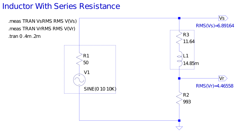
You can download the LTSpice schematic and plot setup.
7.1.1. Ignoring Series Resistance
subs({R=993, R__L=11.64, f=10e3, V__S=6.88458, V__R=4.98893}, inductor_ideal);
L = 0.01502901814
7.1.2. With Series Resistance
subs({R=993, R__L=11.64, f=10e3, V__S=6.88458, V__R=4.98893}, inductor_series_resistance);
L = 0.01483177169
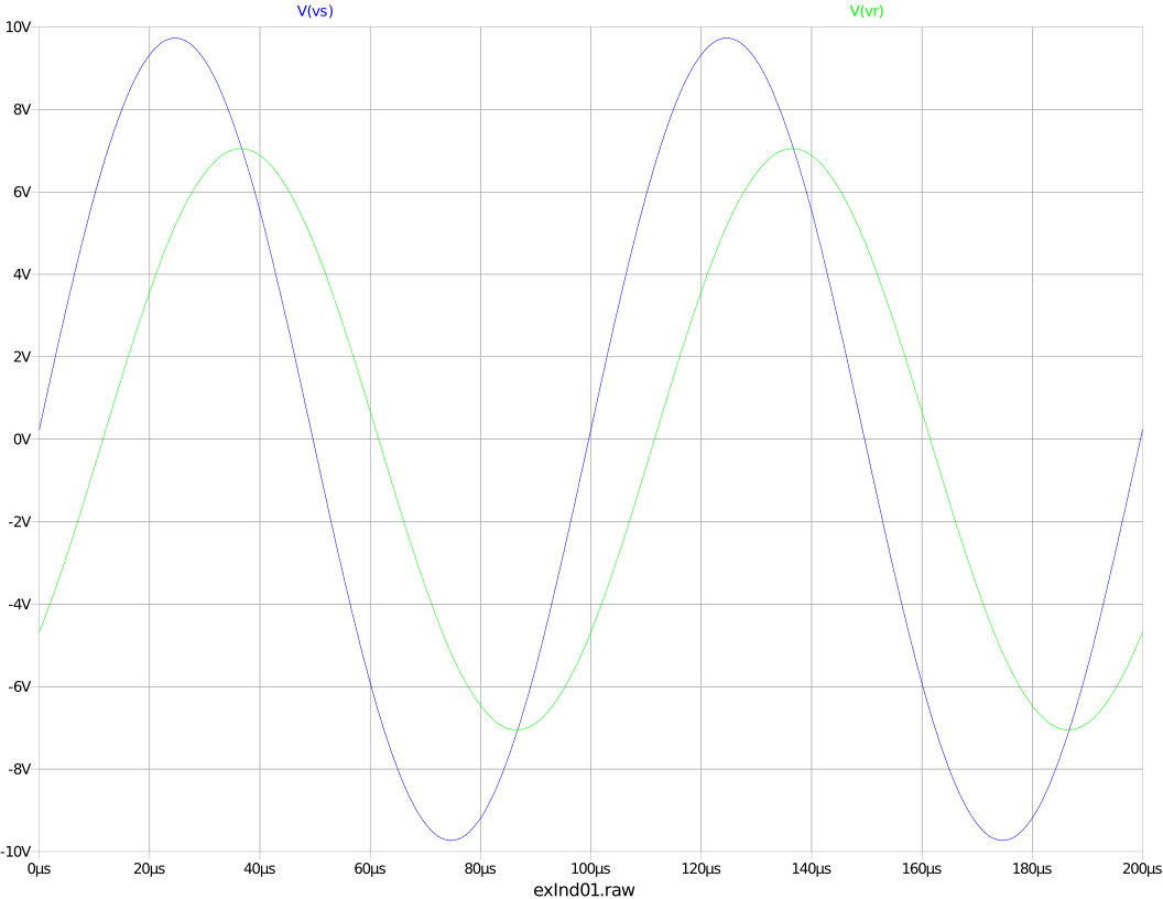
7.1.3. Voltage Plot
Here is a plot of the voltages over time
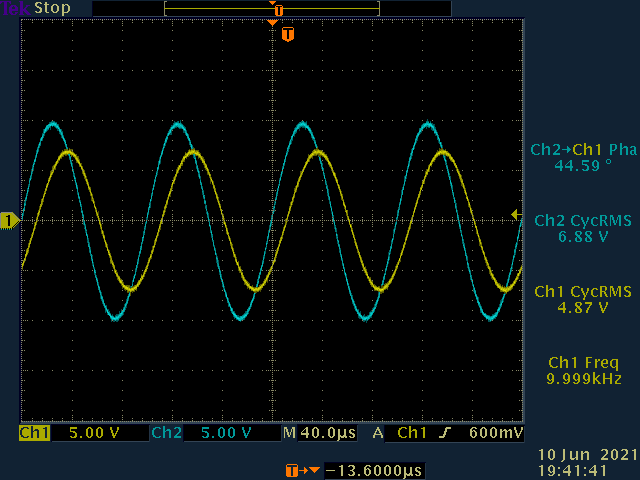
7.1.4. Real Hardware
| Simulation | Tektronix TDS3052B | Siglent SDS2504X | Keysight 34401A | Sanwa Em7000 | |
|---|---|---|---|---|---|
| \(V_S\) | 6.88458 | 6.88 | 6.6523709 | 6.8644 | 6.85 |
| \(V_R\) | 4.98893 | 4.87 | 4.7111941 | 4.8826 | 4.85 |
| \(f\) | 10000 | 9999 | 10001.682 | 9999 | 10000 |
| Phase | 42.9147 | 44.59 | 43.681 | N/A | N/A |
| \(L\) mH | 14.83 | 15.58 | 15.56 | 15.43 | 15.57 |
| %ERR | 0.1% | 4.9% | 4.8% | 3.9% | 4.8% |
7.1.4.1. Tektronix TDS3052B
7.1.4.2. Siglent SDS2504X Plus
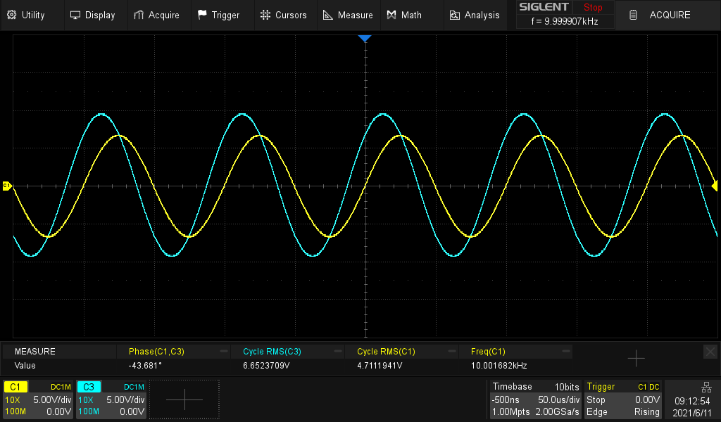
Do not be fooled into thinking the Siglent is more accurate because it prints out more digits. With 10 bits of vertical resolution the answer can only be considered accurate to a bit more than one digit. Paying attention to such details is one of the advantages of the TDS3052B vs the SDS2504X+.
7.1.5. Using Phase Difference
The procedure I have outlined above is to measure the series resistance, and then use the magnitude of the voltages to compute the inductance. This allows us to use a simple voltmeter instead of an oscilloscope. If one can measure the phase difference, then we have another path because it is possible to compute both the inductance and series resistance from the magnitude of the voltages and the phase difference between the two.
7.1.5.1. Exercise
The math is a bit more complex, pun intended. Give it a try. \(V_S=6.89259 \mathrm{V\,RMS}\), \(V_R=4.46626 \mathrm{V\,RMS}\), and the phase angle between \(V_S\) and \(V_R\) is \(42.9147^{\circ}\).
7.1.5.2. Solution
This is a series circuit so all the currents are the same, \(I\). Lets call our unknown impedance \(Z\). Ohm's law tells us \(V_S=I(R+Z)\) and \(V_R=IR\), and so we have:
\[Z=R\left(\frac{V_S}{V_R}-1\right)\]
So we plug \(V_S=6.88458\) and \(V_R= (4.98893\;\angle -42.9147^{\circ}) = 4.98893 e^\frac{-i 2 \pi 42.9147}{360}\) into the above, and get
\[Z = 10.647102 + 939.6345587 i\]
Thus the series resistance is
\[R = \Re(Z) = 10.647102\,\Omega\]
And inductance is:
\[L=\frac{\Im(Z)}{2 \pi f} = 0.01495474847\,\mathrm{H} = 14.95474847\,\mathrm{mH}\]
7.2. Capacitor
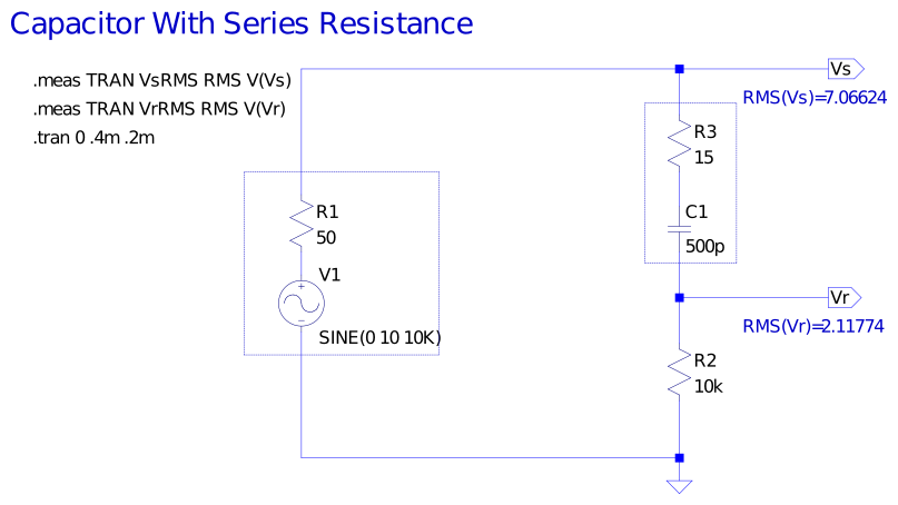
You can download the LTSpice schematic and plot setup.
7.2.1. Ignoring Series Resistance
subs({R=10e3, R__CS=15, f=10e3, V__S=7.06624, V__R=2.11774}, capacitor_ideal);
C = 4.999660552e-10
7.2.2. With Series Resistance
subs({R=10e3, R__CS=15, f=10e3, V__S=7.06624, V__R=2.11774}, capacitor_series_resistance);
C = 5.000401340e-10
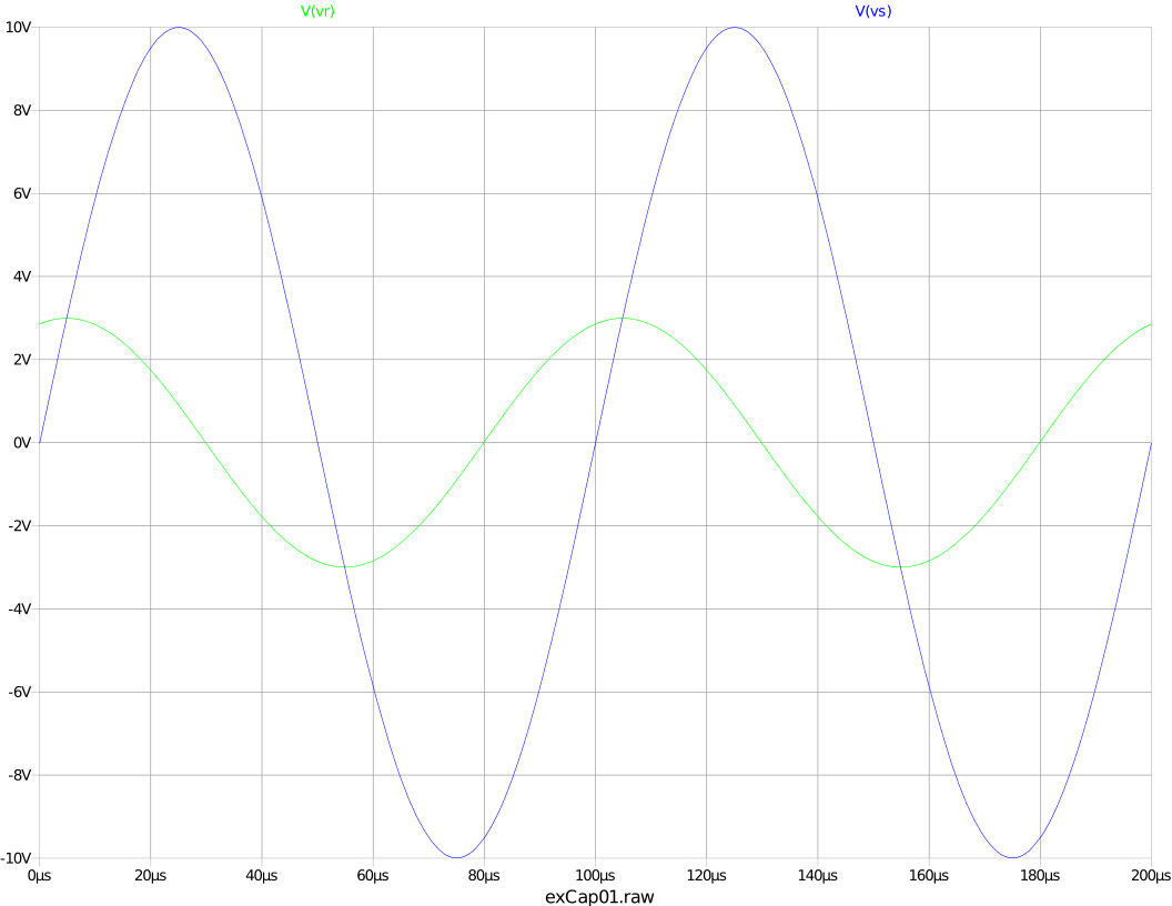
7.2.3. Voltage Plot
Here is a plot of the voltages over time
8. Doing The Math
The algebra can be a bit painful, so here is a bit of maple code that might help. In addition you will find R code for each equation. You can download
the maple code and a PDF version of the maple code.
8.1. Ideal inductor
eq := abs(V__R/R) = abs(V__S/(R+2*Pi*I*f*L));
sol := solve(eq, L) assuming V__R>0, V__S>0, R>0, L>0, f>0;
inductor_ideal := L=simplify(sol[1]); latex(%); CodeGeneration[R](rhs(inductor_ideal), resultname="RCode");
L = sqrt(V_S^2-V_R^2)*R/f/V_R/2.0/pi
\[ L = \frac{\sqrt{-V_{R}^{2}+V_{S}^{2}}\, R}{2 \pi f V_{R}} \]
8.2. Ideal capacitor
eq := abs(V__R/R) = abs(V__S/(R+1/(2*Pi*I*f*C)));
sol := solve(eq, C) assuming V__R>0, V__S>0, R>0, C>0, f>0;
capacitor_ideal := C=simplify(sol[2]); latex(%); CodeGeneration[R](rhs(capacitor_ideal), resultname="RCode");
C = V_R/sqrt(V_S^2-V_R^2)/pi/f/R/2.0
\[ C = \frac{V_{R}}{2 \pi \sqrt{-V_{R}^{2}+V_{S}^{2}}\, f R} \]
8.3. Inductor with series resistance
eq := abs(V__R/R) = abs(V__S/(R+R__L+2*Pi*I*f*L));
sol := solve(eq, L) assuming V__R>0, V__S>0, R>0, L>0, f>0, R__L>0;
inductor_series_resistance := L=simplify(sol[1]); latex(%);  CodeGeneration[R](rhs(inductor_series_resistance), resultname="RCode");
L = sqrt(R^2*V_S^2-(R+R_L)^2*V_R^2)/f/V_R/2.0/pi
\[ L = \frac{\sqrt{-\left(R +R_{L} \right)^{2} V_{R}^{2}+R^{2} V_{S}^{2}}}{2 \pi f V_{R}} \]
8.4. Capacitor with series resistance
eq := abs(V__R/R) = abs(V__S/(R+R__CS+1/(2*Pi*I*f*C))); eq := evalc(eq):
sol := solve(eq, C) assuming V__R>0, V__S>0, R>0, L>0, f>0, R__CS>0;
capacitor_series_resistance := C=simplify(sol[2]); latex(%);  CodeGeneration[R](rhs(capacitor_series_resistance), resultname="RCode");
C = V_R/sqrt(R^2*V_S^2-(R+R_CS)^2*V_R^2)/f/2.0/pi
\[ C = \frac{V_{R}}{2 \pi \sqrt{-\left(R +R_{\mathit{CS}} \right)^{2} V_{R}^{2}+R^{2} V_{S}^{2}}\, f} \]
8.5. Capacitor with parallel resistance
eq := abs(V__R/R) = abs(V__S/(R+1/(1/R__CP+2*Pi*I*f*C))); eq := evalc(eq):
sol := solve(eq, C) assuming V__R>0, V__S>0, R>0, L>0, f>0, R_CP>0;
capacitor_parallel_resistance := C=simplify(sol[1]); latex(%); CodeGeneration[R](rhs(capacitor_parallel_resistance), resultname="RCode");
C = sqrt(2*(R^2+R*R_CP+R_CP^2/2)*V_S^2*V_R^2-V_S^4*R^2-(R+R_CP)^2*V_R^4)/(V_R^2-V_S^2)/f/R/R_CP/2.0/pi
\[ C = \frac{\sqrt{-\left(R +R_{\mathit{CP}} \right)^{2} V_{R}^{4}+2 \left(R^{2}+R R_{\mathit{CP}} +\frac{1}{2} R_{\mathit{CP}}^{2}\right) V_{S}^{2} V_{R}^{2}-V_{S}^{4} R^{2}}}{2 \pi \left(V_{R}^{2}-V_{S}^{2}\right) f R R_{\mathit{CP}}} \]
8.6. Machine Readable Formulas
Below are some machine readable formulas to assist you in doing calculations or for incorporating into your own programs. Some things to note:
- The syntax is Emacs
calcmode which is similar to many infix languages - I removed the underscores from the variable names for broader language support
- "
^" is for exponents - "
sqrt" is the square root. It should always be positive in these calculations, so no need for complex numbers - "
pi" is the constant \(\pi\) - Floating point constants have a decimal point (i.e. 2.0 instead of 2). Integers have no decimal.
- These are not optimized in any way
Emacs users: If you are reading the HTML version of this document, then you may not realize this document was generated from an org-mode file by Emacs. In
the original org-mode document the following are named code blocks which may be called from within Emacs.
Ideal inductor
L = sqrt(VS^2-VR^2)*R/f/VR/2.0/pi
Ideal capacitor
C = VR/sqrt(VS^2-VR^2)/pi/f/R/2.0
Inductor with series resistance
L = sqrt(R^2*VS^2-(R+RL)^2*VR^2)/f/VR/2.0/pi
Capacitor with series resistance
C = VR/sqrt(R^2*VS^2-(R+RCS)^2*VR^2)/f/2.0/pi
Capacitor with parallel resistance
C = sqrt(2*(R^2+R*RCP+RCP^2/2.0)*VS^2*VR^2-VS^4*R^2-(R+RCP)^2*VR^4)/(VR^2-VS^2)/f/R/RCP/2.0/pi