Mitch Richling: Newton Fractal
| Author: | Mitch Richling |
| Updated: | 2024-02-09 |
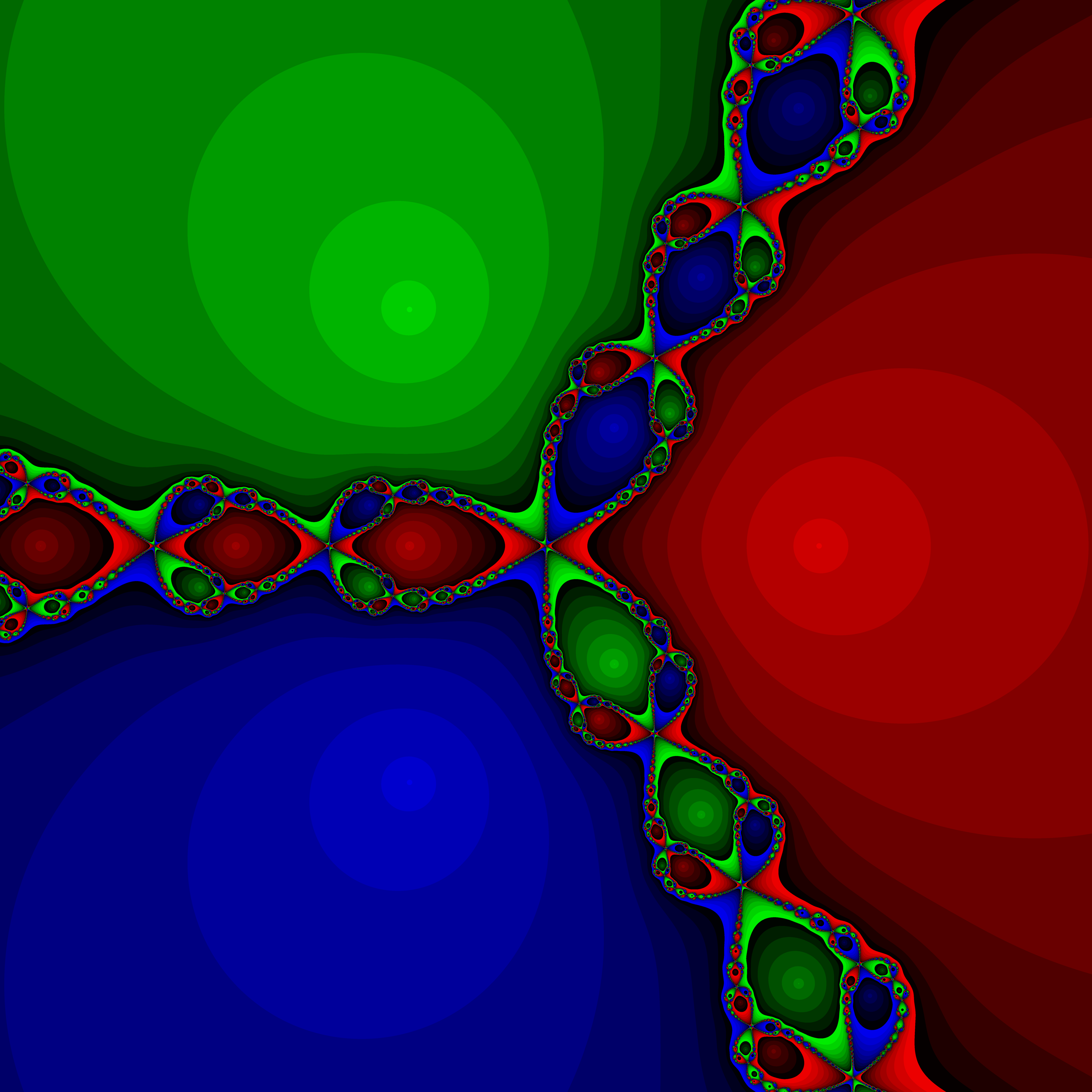
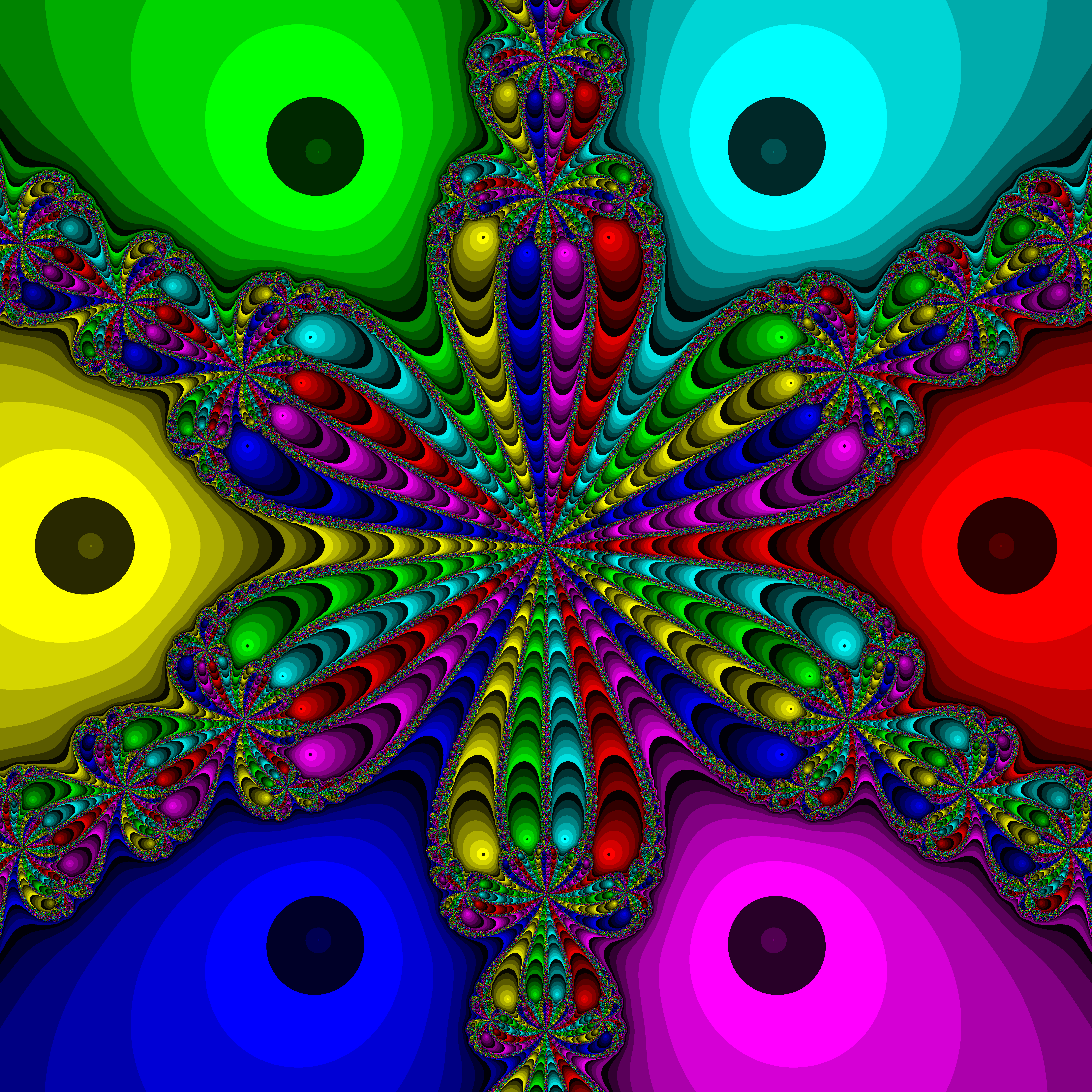
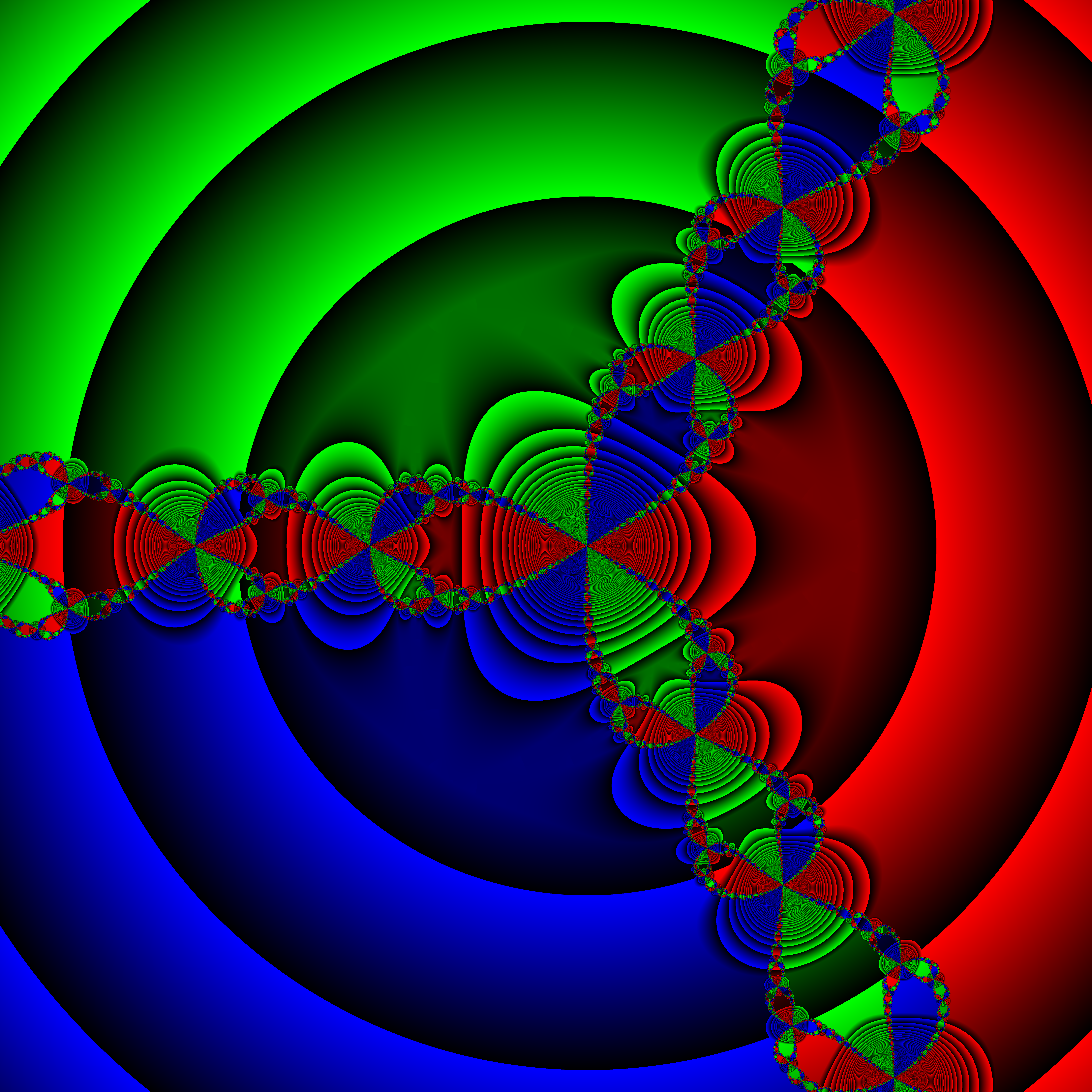
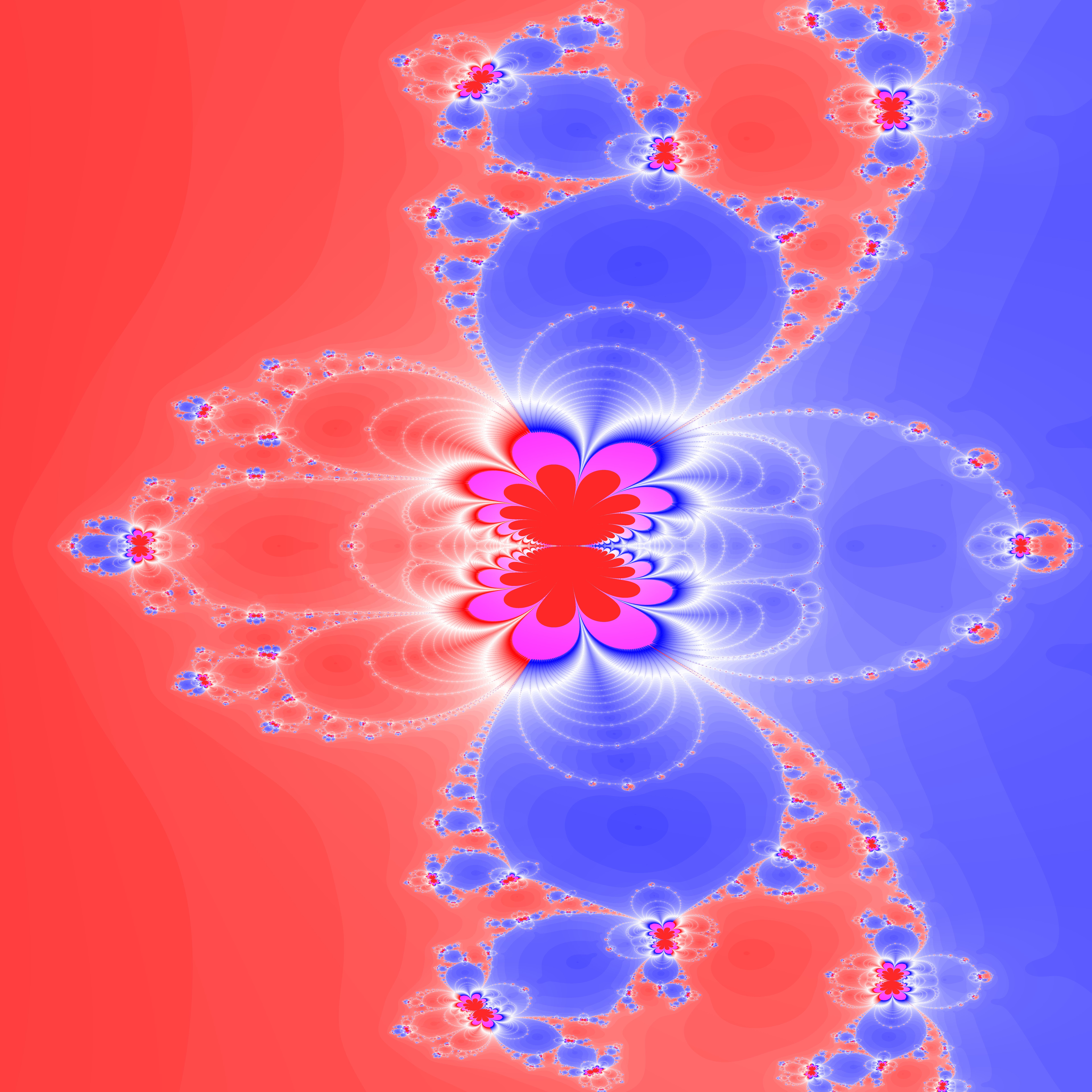
Table of Contents
- 1. Introduction
- 2. The Traditional Newton's Fractal
- 3. Newton's Fractal colored by orbit maximum modulus
- 4. Newton's Fractal colored by distance to other roots
- 5. Newton's Fractal colored by backward progress
- 6. Newton's Fractal colored by angle
- 7. An Orbit Histogram of Newton's Fractal
- 8. Adding poles to the standard case
- 9. Newton's Method applied to a 6th degree polynomial
- 10. Adding poles to the 6th degree case
- 11. Newton's Method applied to non-polynomials
- 12. Modified Newton's Fractals
- 13. Moving beyond Newton: Laguerre's Method
- 14. Laguerre's method with poles
- 15. Code
- 16. References
1. Introduction
While the Mandelbrot set may be the most famous fractal image, the so called "Newton's Fractal" is not too far behind in recognizably. The fractal is a byproduct of an algorithm known as "Newton's method". In mathematical terms, Newton's method takes a function with an initial guess for a root, and specifies a method of constructing an infinite sequence that frequently converges to some root of the function. The fine print for Newton's algorithm surrounds the words "frequently" and "some" in the previous sentence! It can be very difficult to tell if an initial guesses will lead to a root, and to which root it might converge! Knowing that Newton's method converges for a given initial guess tells us almost nothing about the convergence properties for other initial guesses - even ones infinitely close.
For any function we might choose, we may use Newton's method to construct a sequence for any point in the complex plane by using that point as the initial guess for Newton's method. We may then use the convergence properties for each point in the complex plane to draw a picture. This is very similar to the way a sequence convergence pattern is used to draw the Mandelbrot set. The classical Newton's fractal is obtained by drawing the convergence pattern of Newton's method applied to the following function:
\[f(x)=z^3-1\]
If a sequence generated by applying Newton's method to this function converges, then it will be to one of the three cube roots of -1. Because of this, the shading method for Newton's Fractal is a bit more complex than it is for the Mandelbrot set (where we only care about a sequence being bounded or not). For the classic Newton's fractal, we color each point according to which limit point the sequence converges.
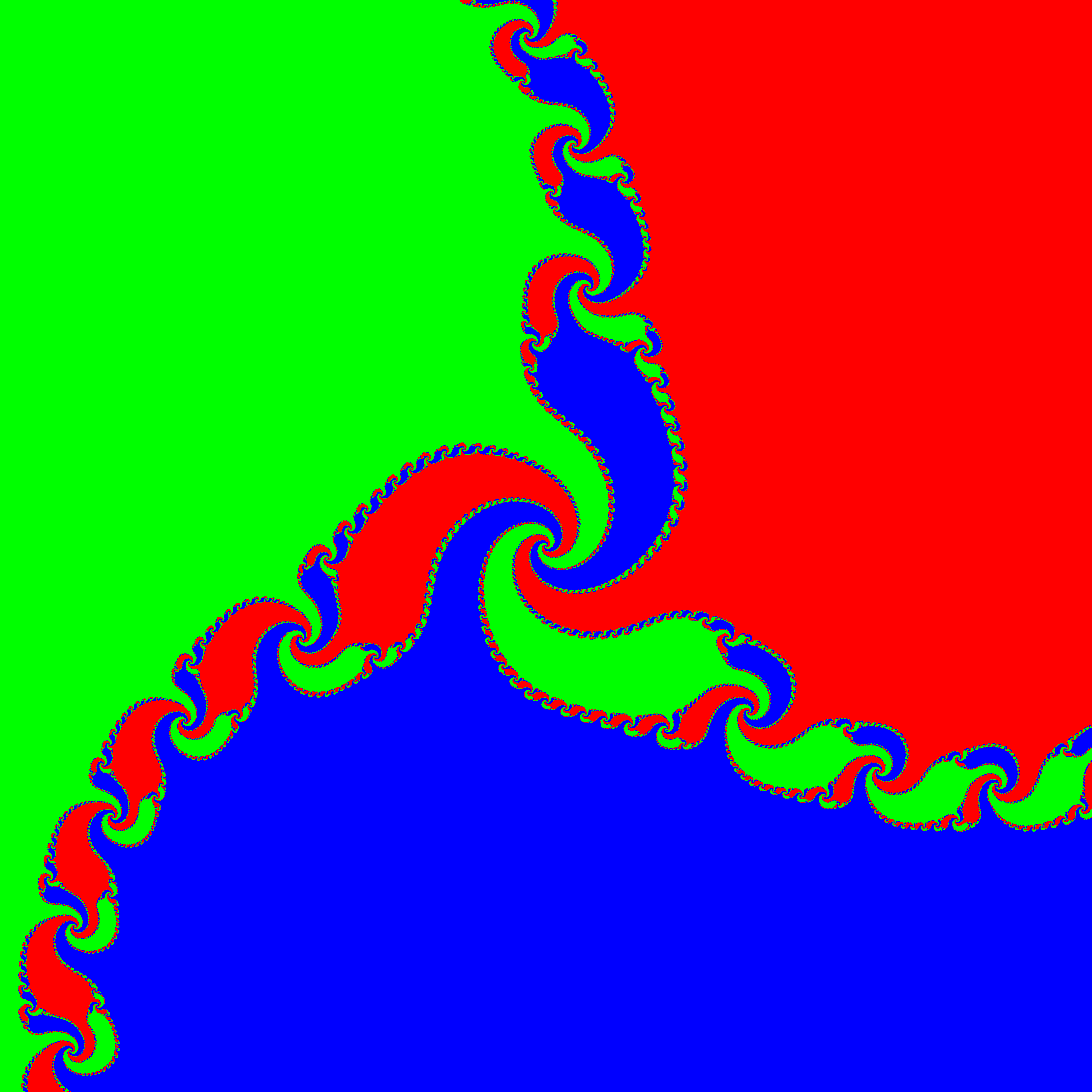
2. The Traditional Newton's Fractal
One can generate Newton's Fractal as normally presented with just a little bit of code. We color a point red if it converges to the real cube root of -1, green if it converges to the complex root in the upper half-plane, blue if it converges to the complex root in the lower half-plane, and we leave the point black if it doesn't converge at all. The shade of red, blue, or green is determined by how fast the sequence appeared to converge to the appropriate root - brighter colors mean faster convergence.
#include "ramCanvas.hpp"

int main(void) {
  std::chrono::time_point<std::chrono::system_clock> startTime = std::chrono::system_clock::now();
  const int            MAXITR = 255;
  const int            COLMAG = 25;
  const double         ZROEPS = .0001;
  const int            IMGSIZ = 7680;
  std::complex<double> r1( 1.0,                        0.0);
  std::complex<double> r2(-0.5,  sin(2*std::numbers::pi/3));
  std::complex<double> r3(-0.5, -sin(2*std::numbers::pi/3));
  mjr::ramCanvas3c8b   theRamCanvas(IMGSIZ, IMGSIZ, -2.0, 2, -2, 2); // -0.9, -0.7, -0.1, 0.1

# pragma omp parallel for schedule(static,1)
  for(int y=0;y<theRamCanvas.getNumPixY();y++) {
    for(int x=0;x<theRamCanvas.getNumPixX();x++) {
      std::complex<double> z = theRamCanvas.int2real(x, y);
      for(int count=0; count<MAXITR; count++) {
        if(std::abs(z-r1) <= ZROEPS) {
          theRamCanvas.drawPoint(x, y, mjr::ramCanvas3c8b::colorType::csCCu0R::c(255-count*COLMAG)); break;
        } else if(std::abs(z-r2) <= ZROEPS) {
          theRamCanvas.drawPoint(x, y, mjr::ramCanvas3c8b::colorType::csCCu0G::c(255-count*COLMAG)); break;
        } else if(std::abs(z-r3) <= ZROEPS) {
          theRamCanvas.drawPoint(x, y, mjr::ramCanvas3c8b::colorType::csCCu0B::c(255-count*COLMAG)); break;
        } else if(std::abs(z) <= ZROEPS) {
          break;
        }
        z = z-(z*z*z-1.0)/(z*z*3.0);
      }
    }
  }
  theRamCanvas.writeTIFFfile("newton_simple.tiff");
  std::chrono::duration<double> runTime = std::chrono::system_clock::now() - startTime;
  std::cout << "Total Runtime " << runTime.count() << " sec" << std::endl;
}
The above program will generate this picture:
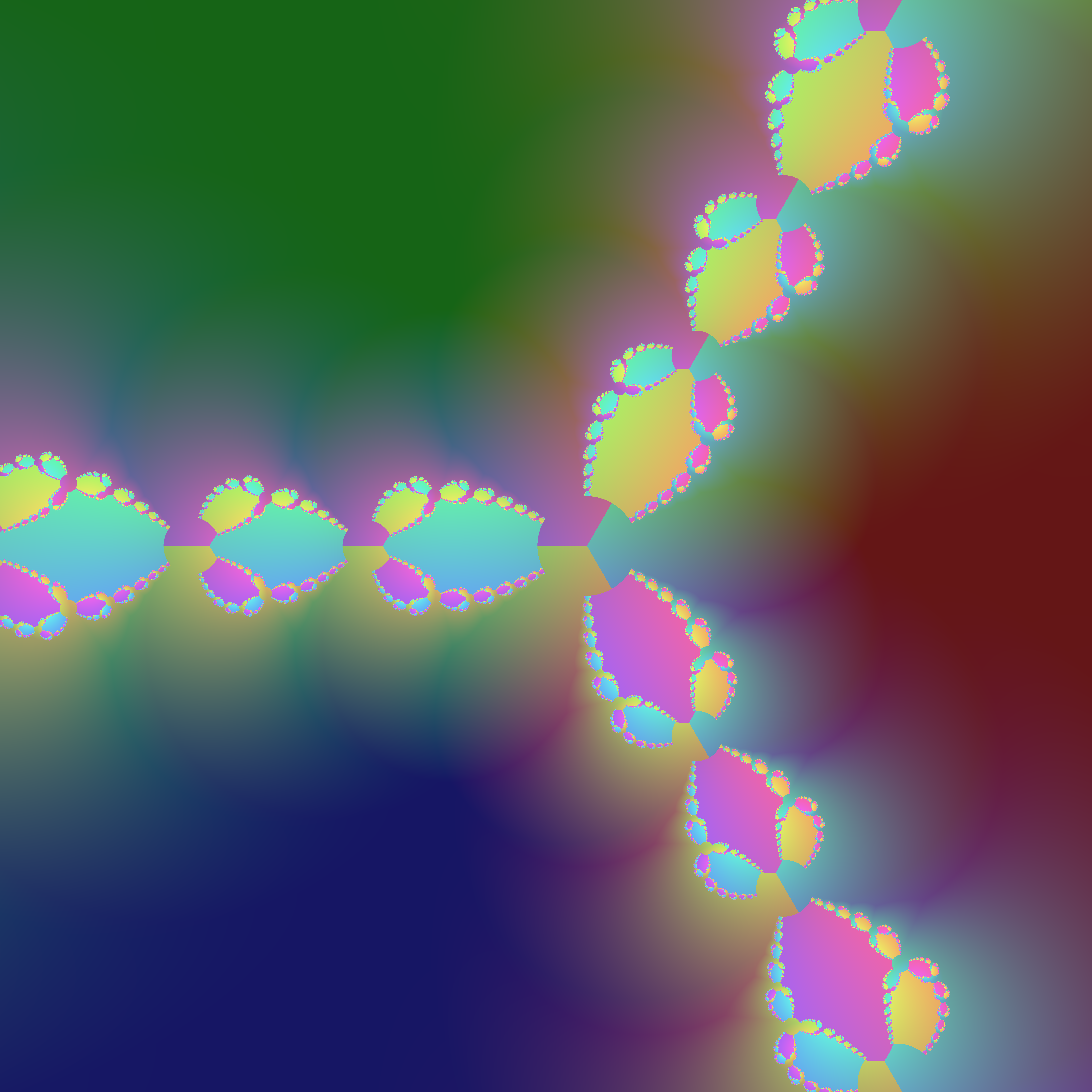
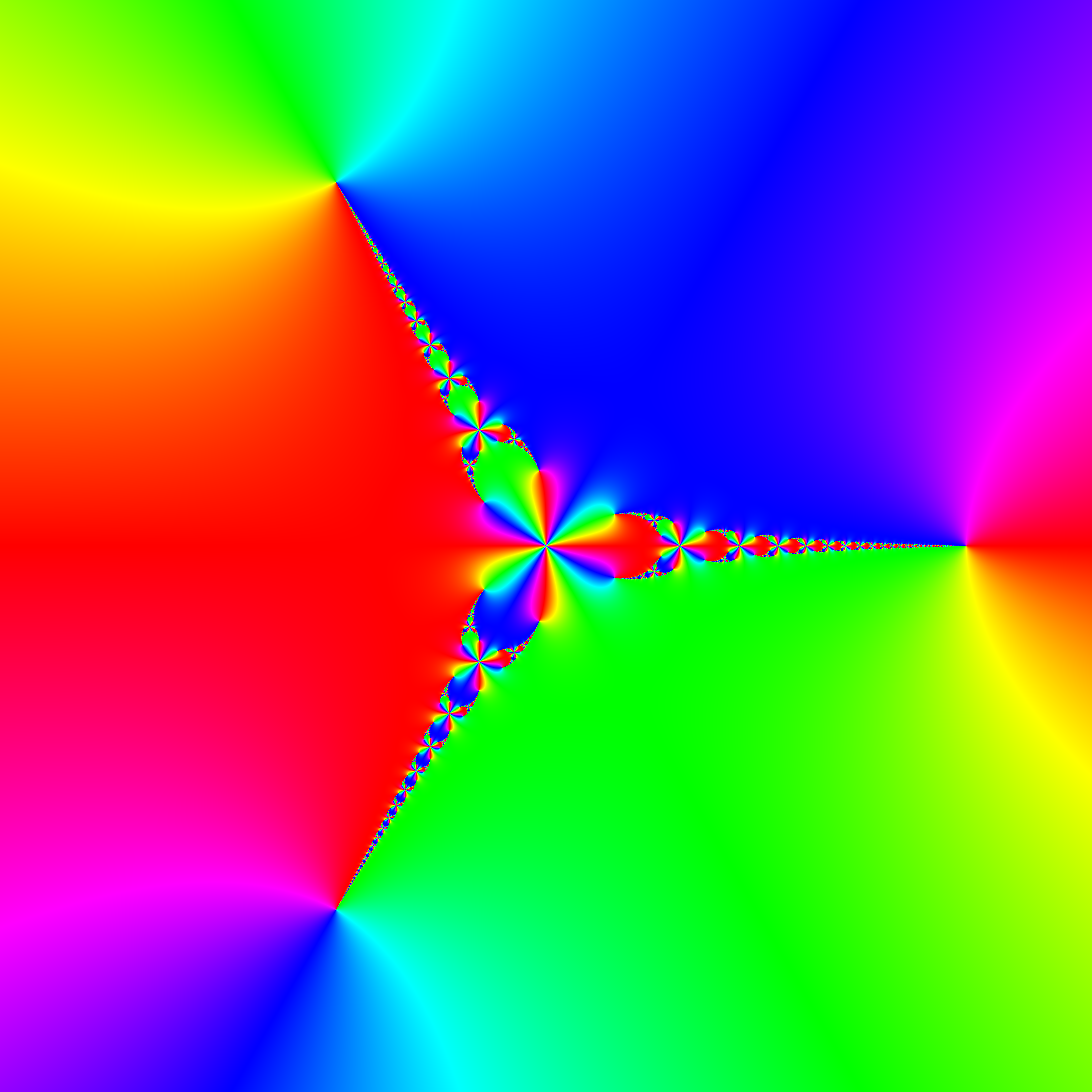
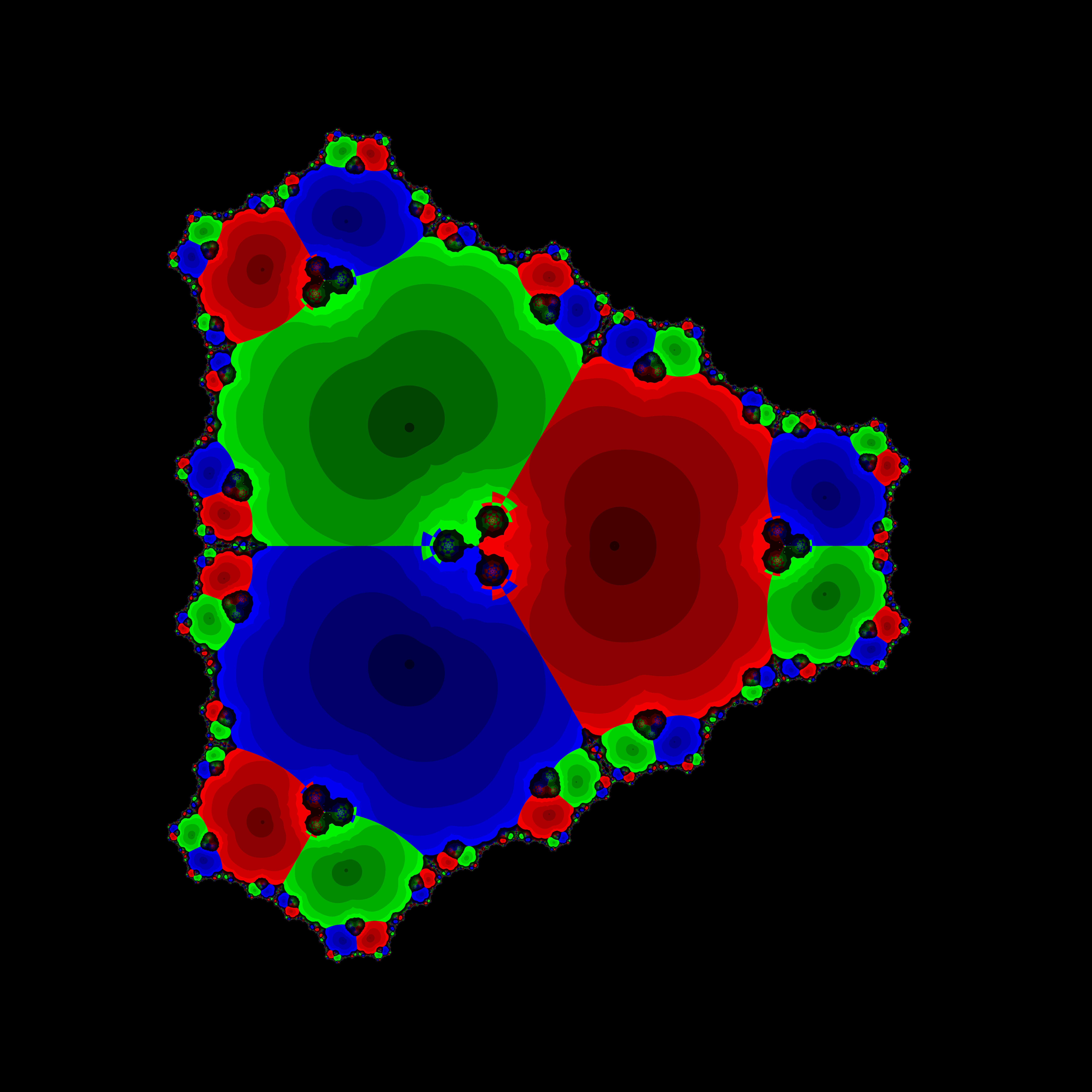
3. Newton's Fractal colored by orbit maximum modulus
Nothing wrong with the traditional way of drawing Newton's fractal; however, some insight into just how strange the convergence is for Newton's method may be obtained from a different coloring algorithm. In the funny regions between roots, it is clear that very tiny disks exist that contain distinct points which converge to each of the three roots. One can see this at the center of the image for example where we see red, blue, and green very near each other. In fact, each place where the "fish" come together to "kiss" contains such a disk. Even knowing such little disks have this behavior doesn't necessarily prepare one for the fact that newton's method doesn't converge very well in such disks – i.e. the sequence doesn't simply start in the disk and make a bee-line for the appropriate root. Instead, the sequence can "blow up" and reach VERY large complex numbers (in modulus) before it begins to behave itself and converges nicely to a root. One can see this strange behavior by coloring the pixels according to the maximum modulus achieved by a sequence on the way to convergence.
This new image may be generated by making a slight modification to the previous program:
#include "ramCanvas.hpp"

typedef mjr::ramCanvas3c8b rcT;  // The Ram Canvas type we will use
typedef rcT::colorType rccT;     // The Ram Canvas color type
typedef rcT::csIntType rccsiT;   // The Ram Canvas color scheme index type

int main(void) {
  std::chrono::time_point<std::chrono::system_clock> startTime = std::chrono::system_clock::now();
  const int            MAXITR = 255;
  const int            COLMAG = 400;
  const double         ZROEPS = .0001;
  const int            IMGSIZ = 7680;
  std::complex<double> r1( 1.0,                        0.0);
  std::complex<double> r2(-0.5,  sin(2*std::numbers::pi/3));
  std::complex<double> r3(-0.5, -sin(2*std::numbers::pi/3));
  rcT                  theRamCanvas(IMGSIZ, IMGSIZ, -2.15, 1.85, -2.0, 2.0);

# pragma omp parallel for schedule(static,1)
  for(int y=0;y<theRamCanvas.getNumPixY();y++) {
    for(int x=0;x<theRamCanvas.getNumPixX();x++) {
      std::complex<double> z = theRamCanvas.int2real(x, y);
      double maxMod = 0.0;
      for(int count=0; count<MAXITR; count++) {
        if(std::abs(z-r1) <= ZROEPS) {
          theRamCanvas.drawPoint(x, y, rccT::csCCu0R::c(static_cast<rccsiT>(255-maxMod*COLMAG))); break;
        } else if(std::abs(z-r2) <= ZROEPS) {
          theRamCanvas.drawPoint(x, y, rccT::csCCu0G::c(static_cast<rccsiT>(255-maxMod*COLMAG))); break;
        } else if(std::abs(z-r3) <= ZROEPS) {
          theRamCanvas.drawPoint(x, y, rccT::csCCu0B::c(static_cast<rccsiT>(255-maxMod*COLMAG))); break;
        } else if(std::abs(z) <= ZROEPS) {
          break;
        }
        if(abs(z)>maxMod)
          maxMod=abs(z);
        z = z-(z*z*z-1.0)/(z*z*3.0);
      }
    }
  }
  theRamCanvas.writeTIFFfile("newton_max_mod.tiff");
  std::chrono::duration<double> runTime = std::chrono::system_clock::now() - startTime;
  std::cout << "Total Runtime " << runTime.count() << " sec" << std::endl;
}
The above program will generate this picture:
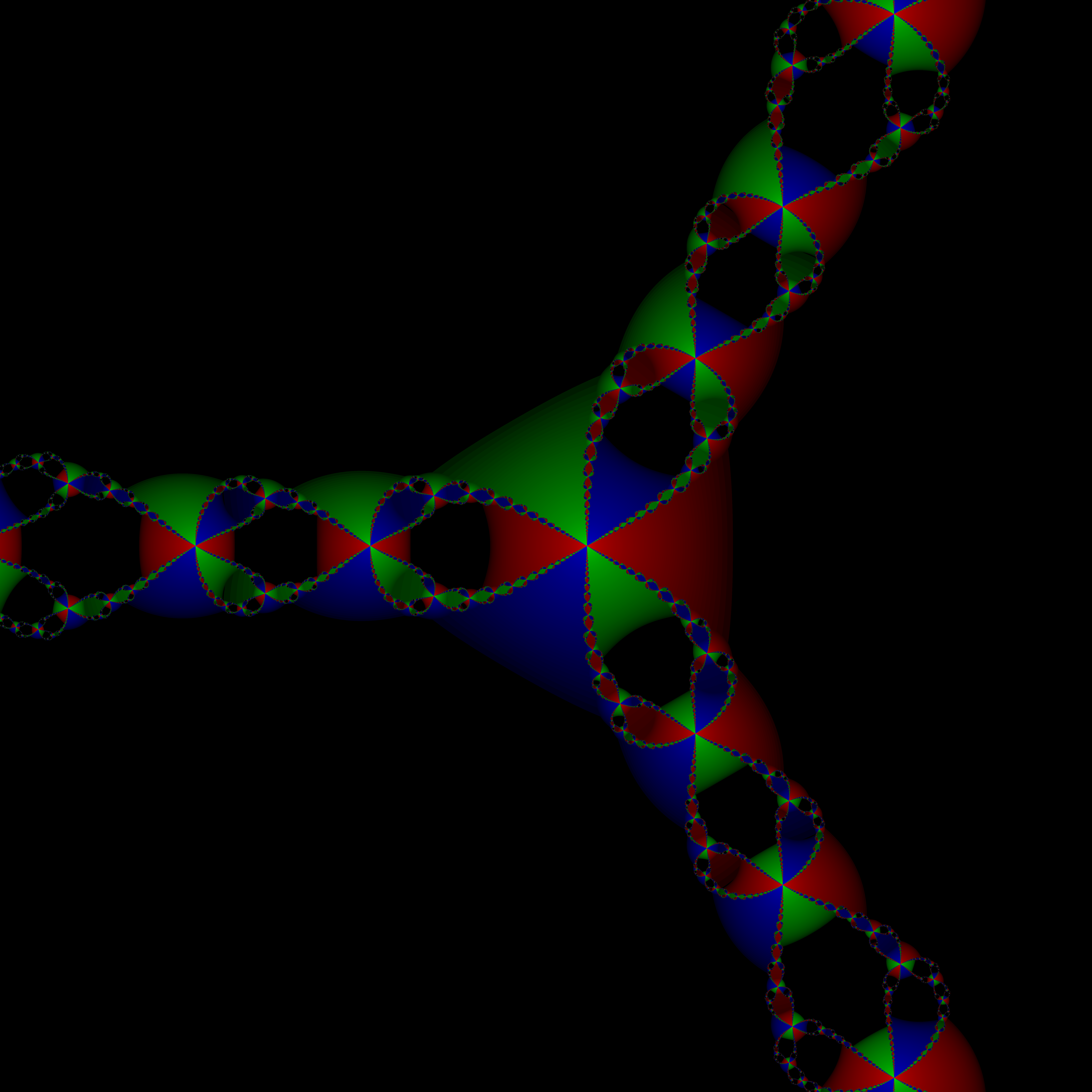
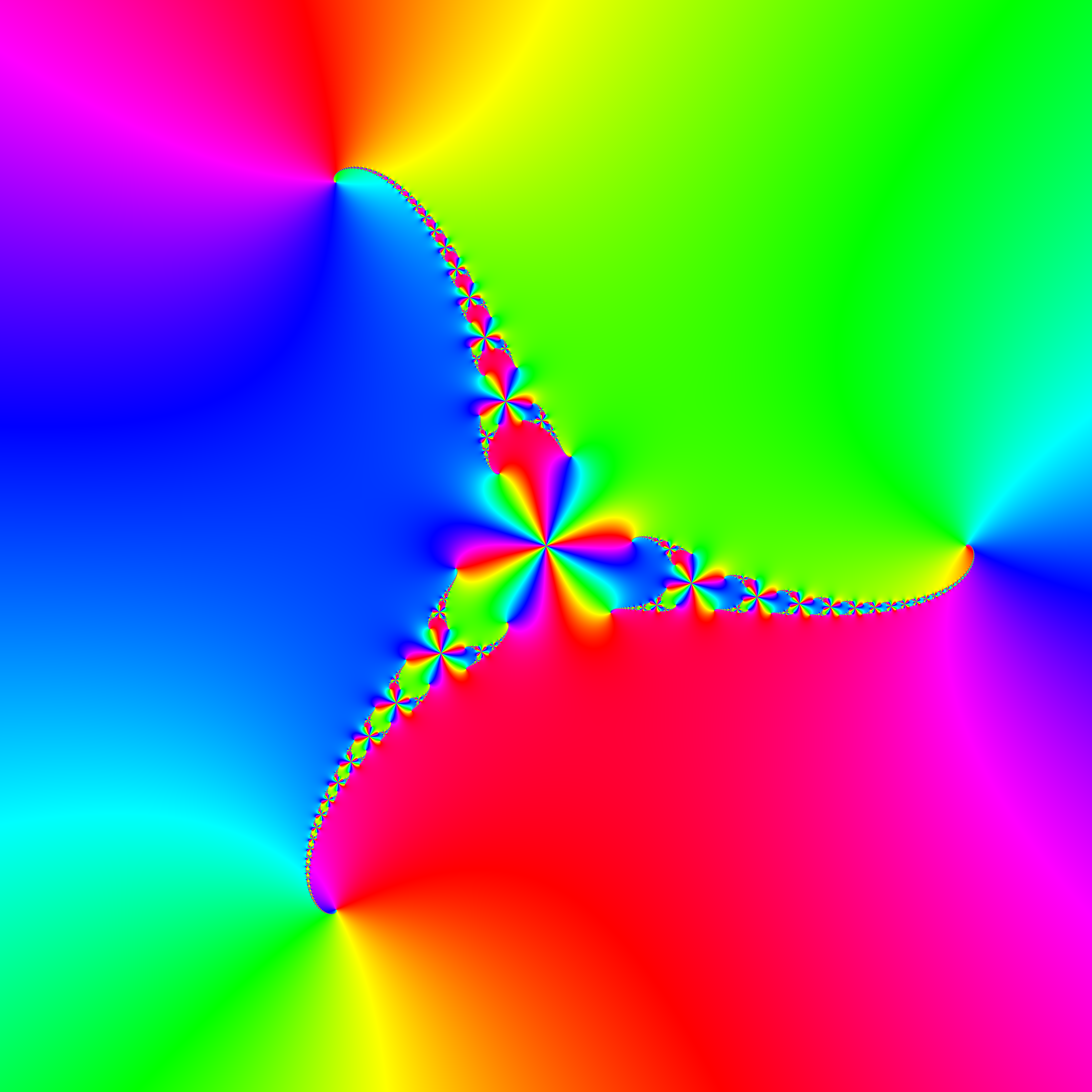
4. Newton's Fractal colored by distance to other roots
Continuing the investigation of how Newton's method converges, we color the points according to how close the orbit of each point gets to the roots to which it doesn't converge.
This new image may be generated by making a slight modification to the previous program:
#include "ramCanvas.hpp"

typedef mjr::ramCanvas3c8b rcT;      // The Ram Canvas type we will use
typedef rcT::colorChanType rcccT;    // Color Channel Type

int main(void) {
  std::chrono::time_point<std::chrono::system_clock> startTime = std::chrono::system_clock::now();
  int                  MAXITR = 255;
  double               ZROEPS = .0001;
  double               MAXZ   = 10;
  const int            IMGSIZ = 7680;
  std::complex<double> r1( 1.0,                        0.0);
  std::complex<double> r2(-0.5,  sin(2*std::numbers::pi/3));
  std::complex<double> r3(-0.5, -sin(2*std::numbers::pi/3));
  rcT                  theRamCanvas(IMGSIZ, IMGSIZ, -2.15, 1.85, -2.0, 2.0);

# pragma omp parallel for schedule(static,1)
  for(int y=0;y<theRamCanvas.getNumPixY();y++) {
    for(int x=0;x<theRamCanvas.getNumPixX();x++) {
      std::complex<double> z = theRamCanvas.int2real(x, y);
      double minMod1 = std::abs(z-r1);
      double minMod2 = std::abs(z-r2);
      double minMod3 = std::abs(z-r3);
      for(int count=0; count<MAXITR; count++) {
        double modz = std::abs(z);
        if ((modz>MAXZ) || (modz<ZROEPS))
          break;
        z = z-(z*z*z-1.0)/(z*z*3.0);
        if(std::abs(z-r1) < minMod1) minMod1 = std::abs(z-r1);
        if(std::abs(z-r2) < minMod2) minMod2 = std::abs(z-r2);
        if(std::abs(z-r3) < minMod3) minMod3 = std::abs(z-r3);
        if ((modz<ZROEPS) || (minMod1<ZROEPS) || (minMod2<ZROEPS) || (minMod3<ZROEPS))
          break;
      }

      rcccT r = static_cast<rcccT>((minMod1 < std::min(minMod2, minMod3) ? 100.0 : 720.0*std::log(4.73-minMod1)));
      rcccT g = static_cast<rcccT>((minMod2 < std::min(minMod1, minMod3) ? 100.0 : 720.0*std::log(4.73-minMod2)));
      rcccT b = static_cast<rcccT>((minMod3 < std::min(minMod1, minMod2) ? 100.0 : 720.0*std::log(4.73-minMod3)));
      theRamCanvas.drawPoint(x, y, rcT::colorType(r, g, b));
    }
  }

  theRamCanvas.writeTIFFfile("newton_min_root.tiff");
  std::chrono::duration<double> runTime = std::chrono::system_clock::now() - startTime;
  std::cout << "Total Runtime " << runTime.count() << " sec" << std::endl;
}
The above program will generate this picture:
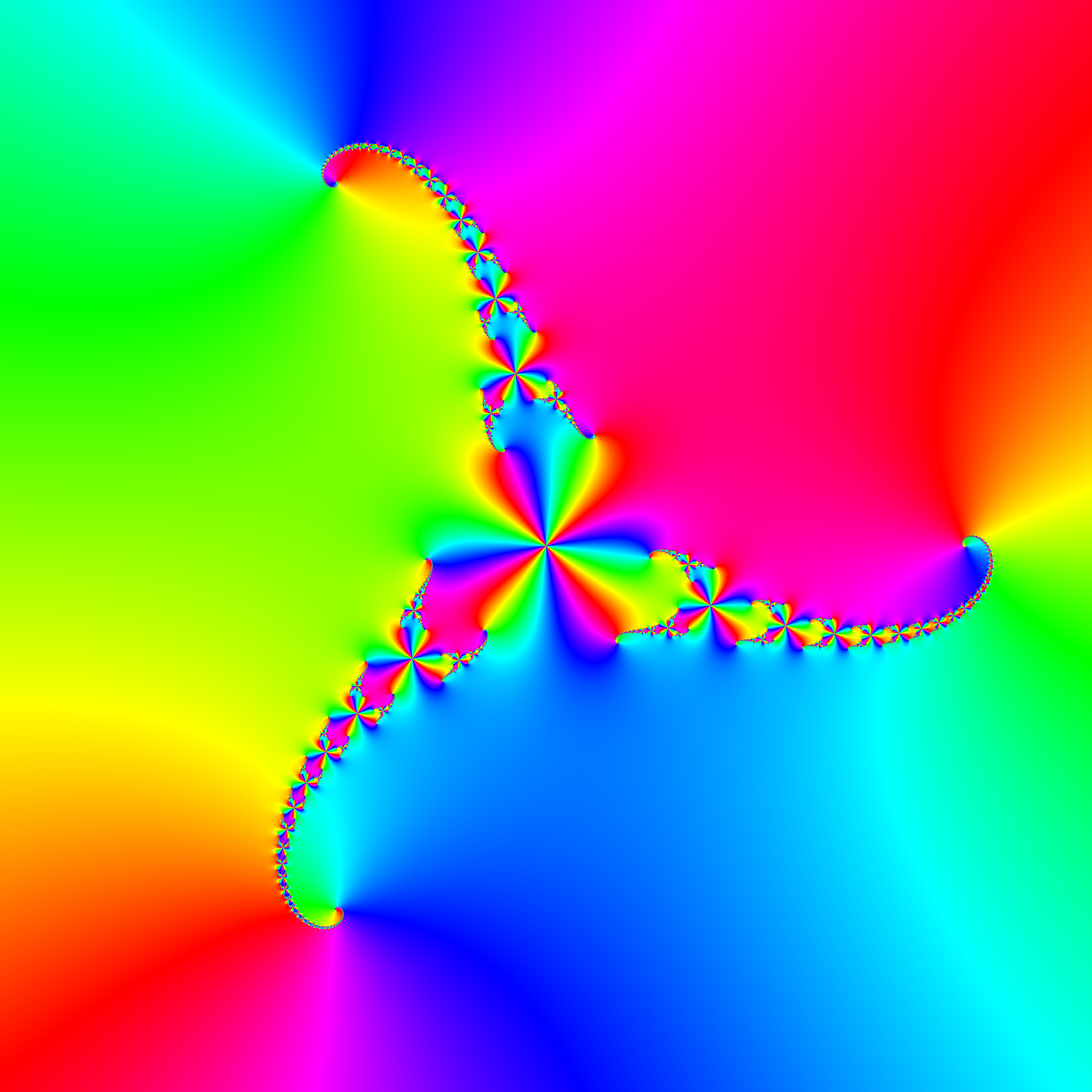
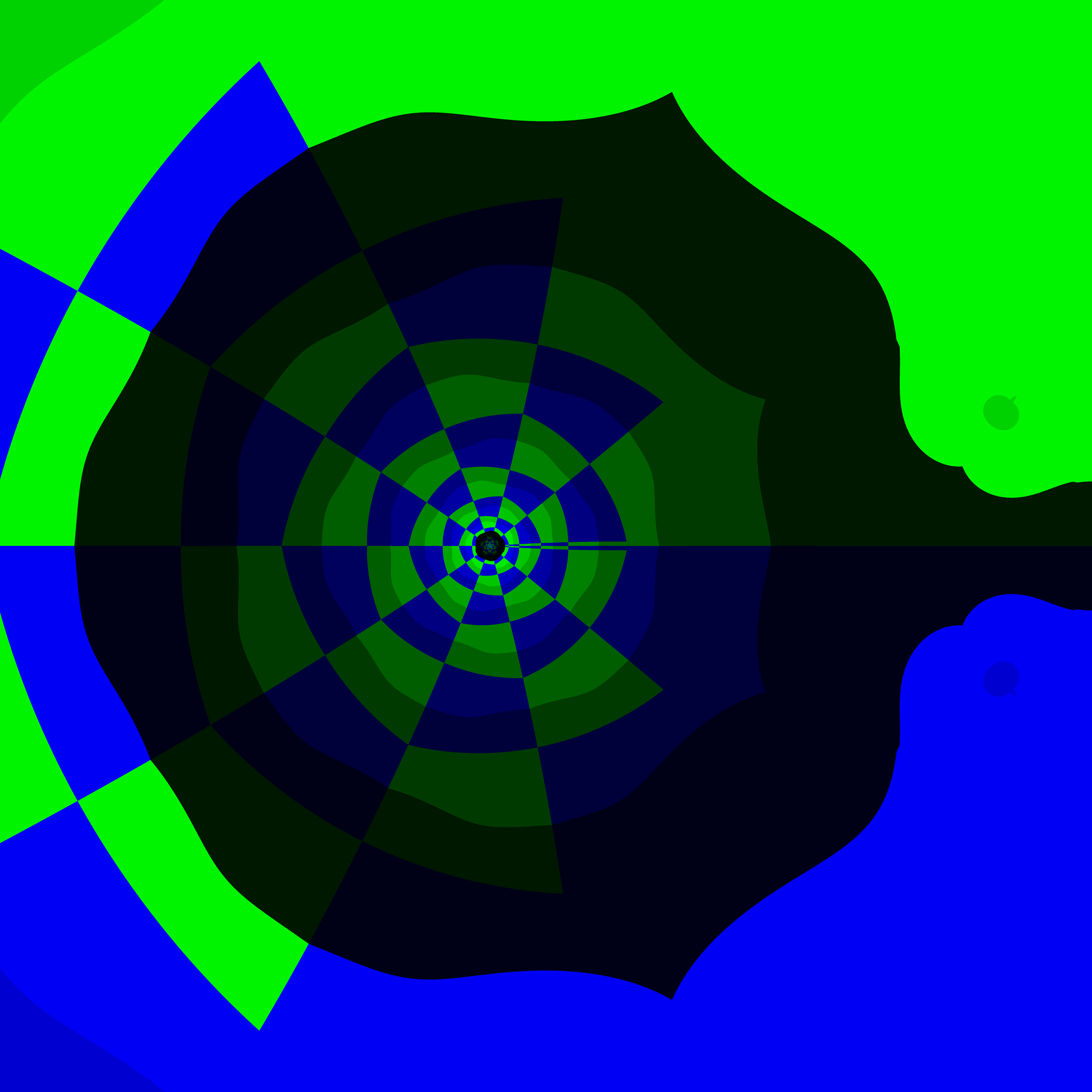
5. Newton's Fractal colored by backward progress
We like to think of Newton's method nicely converging to a root with each iteration getting ever closer. In the section Newton's Fractal colored by orbit maximum modulus we discovered that doesn't happen. SO here we take a closer look at orbits that take steps away from the root to which they converge. Then we color points by the maximum such back-step from the root.
Here is an example starting near the origin:
# -0.000140461 -> 1.68953e+07 -> 1.12635e+07 -> ... (40 steps) ... -> 1.03286 -> 1.00103 #
Here is a bit of code to draw the largest back-steps:
#include "ramCanvas.hpp"

typedef mjr::ramCanvas3c8b rcT;      // The Ram Canvas type we will use
typedef rcT::colorChanType rcccT;    // Color Channel Type

int main(void) {
  std::chrono::time_point<std::chrono::system_clock> startTime = std::chrono::system_clock::now();
  constexpr int        MAXITR = 255;
  constexpr double     ZROEPS = .0001;
  constexpr int        IMGSIZ = 7680;
  std::complex<double> r1( 1.0,                        0.0);
  std::complex<double> r2(-0.5,  sin(2*std::numbers::pi/3));
  std::complex<double> r3(-0.5, -sin(2*std::numbers::pi/3));
  rcT                  theRamCanvas(IMGSIZ, IMGSIZ, -2.15, 1.85, -2.0, 2.0);

# pragma omp parallel for schedule(static,1)
  for(int y=0;y<theRamCanvas.getNumPixY();y++) {
    for(int x=0;x<theRamCanvas.getNumPixX();x++) {
      std::complex<double> z = theRamCanvas.int2real(x, y);
      std::complex<double> zL = z;
      double maxStepBack1 = 0.0;
      double maxStepBack2 = 0.0;
      double maxStepBack3 = 0.0;
      double curRootMod1 = 1.0;
      double curRootMod2 = 1.0;
      double curRootMod3 = 1.0;
      for(int count=0; count<MAXITR; count++) {
        double modz = std::abs(z);
        if (modz<ZROEPS)
          break;
        z = z-(z*z*z-1.0)/(z*z*3.0);
        curRootMod1 = std::abs(z-r1);
        curRootMod2 = std::abs(z-r2);
        curRootMod3 = std::abs(z-r3);
        double curStepBack1 = curRootMod1 - std::abs(zL-r1);
        double curStepBack2 = curRootMod2 - std::abs(zL-r2);
        double curStepBack3 = curRootMod3 - std::abs(zL-r3);
        if(curStepBack1 > maxStepBack1) maxStepBack1 = curStepBack1;
        if(curStepBack2 > maxStepBack2) maxStepBack2 = curStepBack2;
        if(curStepBack3 > maxStepBack3) maxStepBack3 = curStepBack3;
        if ((modz<ZROEPS) || (curRootMod1<ZROEPS) || (curRootMod2<ZROEPS) || (curRootMod3<ZROEPS))
          break;
      }

      rcccT r = static_cast<rcccT>(( ((curRootMod1 < 2*ZROEPS) && (maxStepBack1 > 0)) ? std::log(1+maxStepBack1)*18 : 0));
      rcccT g = static_cast<rcccT>(( ((curRootMod2 < 2*ZROEPS) && (maxStepBack2 > 0)) ? std::log(1+maxStepBack2)*18 : 0));
      rcccT b = static_cast<rcccT>(( ((curRootMod3 < 2*ZROEPS) && (maxStepBack3 > 0)) ? std::log(1+maxStepBack3)*18 : 0));
      theRamCanvas.drawPoint(x, y, rcT::colorType(r, g, b));
    }
  }
  theRamCanvas.autoMaxHistStrechRGB();
  theRamCanvas.applyHomoPixTfrm(&rcT::colorType::tfrmPow, 0.4);
  theRamCanvas.writeTIFFfile("newton_max_back.tiff");
  std::chrono::duration<double> runTime = std::chrono::system_clock::now() - startTime;
  std::cout << "Total Runtime " << runTime.count() << " sec" << std::endl;
}
The above program will generate this picture:
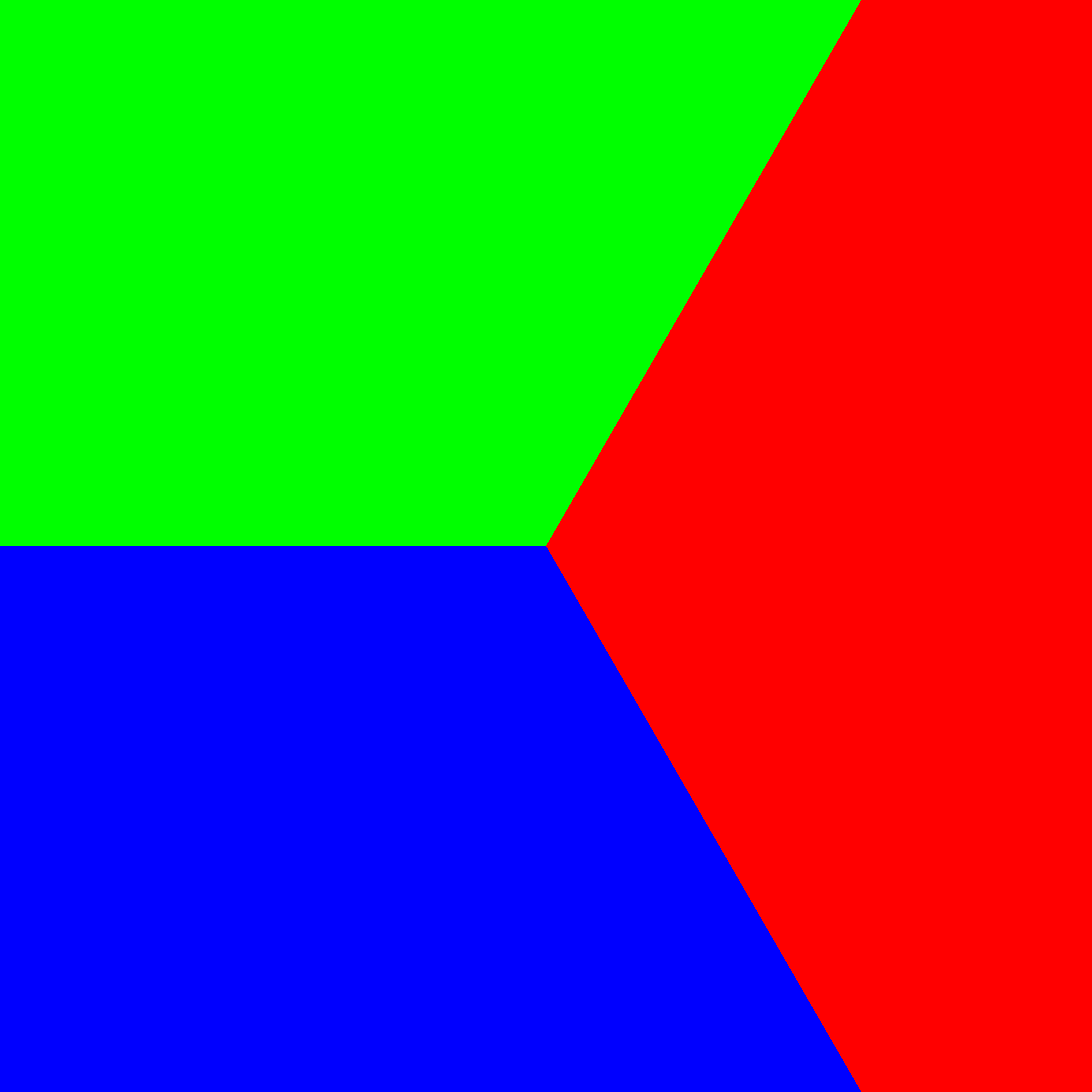
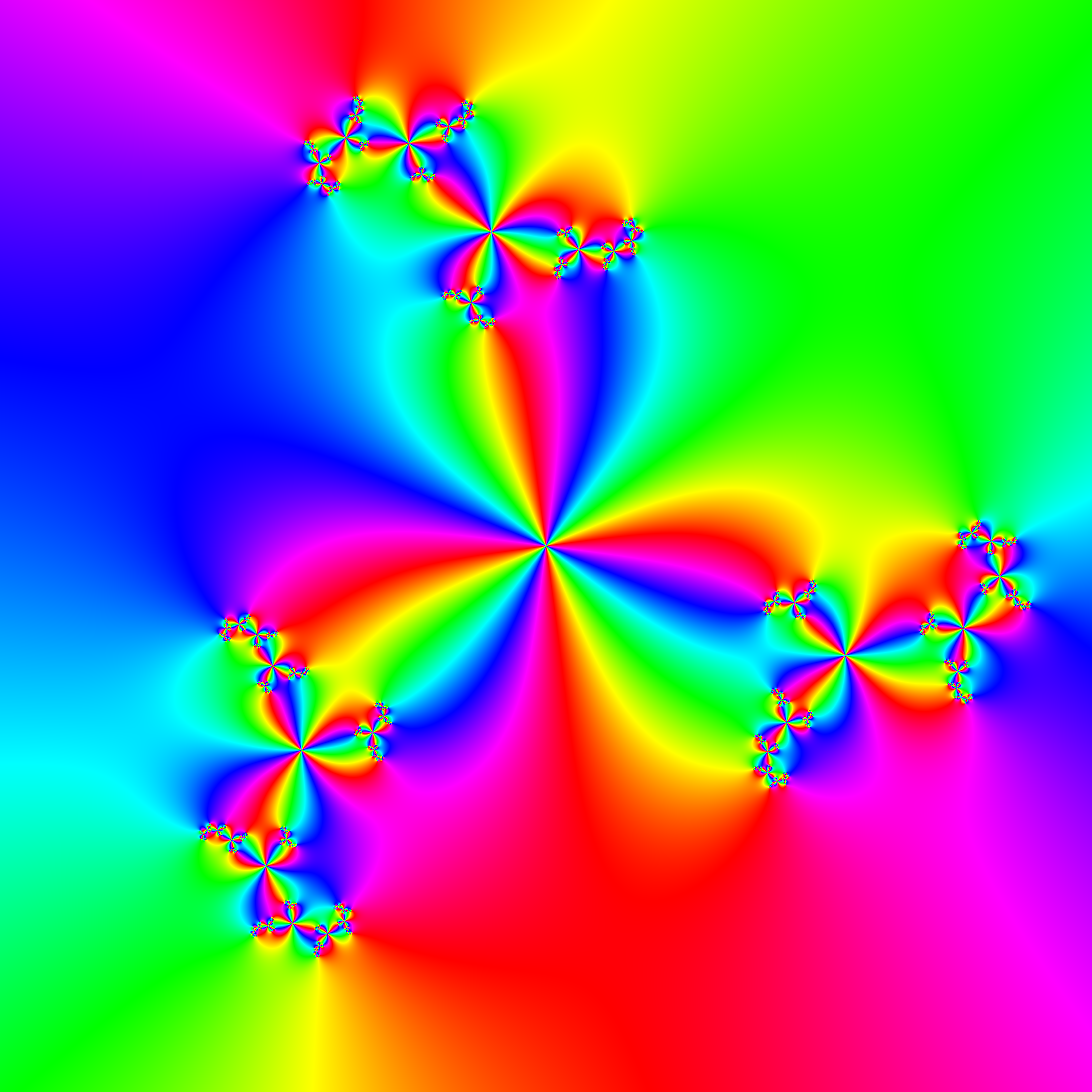
6. Newton's Fractal colored by angle
\(z^2-1\) has three roots located a phase angles of \(0\) and \(\pm\frac{2\pi}{3}\). We can divide up the plane like a pie slicing it three times between these roots like so:
Now we can use these rays from the origin as a kind of orbit trap by keeping track of the minimal phase angle difference between these rays and the newton iterations. We can color things based on which ray was the one that the orbit got closest to, or by the root the orbit converges to. In the code below we use the root:
#include "ramCanvas.hpp"

typedef mjr::ramCanvas3c8b rcT;      // The Ram Canvas type we will use
typedef rcT::colorChanType rcccT;    // Color Channel Type

int main(void) {
  std::chrono::time_point<std::chrono::system_clock> startTime = std::chrono::system_clock::now();
  constexpr int        MAXITR = 255;
  constexpr double     ZROEPS = .0001;
  constexpr int        IMGSIZ = 7680;
  constexpr double     ang1   = 0.0;
  constexpr double     ang2   = 2*std::numbers::pi/3;
  constexpr double     ang3   = -2*std::numbers::pi/3;
  constexpr double     ang12  =  (ang1+ang2)/2.0;
  constexpr double     ang13  =  (ang1+ang3)/2.0;
  constexpr double     ang23  =  std::numbers::pi;
  constexpr double     normer = std::log(2*std::numbers::pi/3);
  std::complex<double> r1( 1.0,  sin(ang1));
  std::complex<double> r2(-0.5,  sin(ang2));
  std::complex<double> r3(-0.5,  sin(ang3));
  rcT                  theRamCanvas(IMGSIZ, IMGSIZ, -2.15, 1.85, -2.0, 2.0);

# pragma omp parallel for schedule(static,1)
  for(int y=0;y<theRamCanvas.getNumPixY();y++) {
    if ((y%100)==0)
#     pragma omp critical
      std::cout << "line " << y << " of " << IMGSIZ << std::endl;
    for(int x=0;x<theRamCanvas.getNumPixX();x++) {
      std::complex<double> z = theRamCanvas.int2real(x, y);
      double minAngleDelta1 = std::numbers::pi;
      double minAngleDelta2 = std::numbers::pi;
      double minAngleDelta3 = std::numbers::pi;
      for(int count=0; count<MAXITR; count++) {
        double modz = std::abs(z);
        if (modz<ZROEPS)
          break;
        z = z-(z*z*z-1.0)/(z*z*3.0);
        double curAngle = std::arg(z);
        double curAngleDelta1 = std::abs(ang12-curAngle);
        double curAngleDelta2 = std::abs(ang13-curAngle);
        double curAngleDelta3 = std::min(std::abs(curAngle-ang23), std::abs(curAngle+ang23));
        if(curAngleDelta1 < minAngleDelta1) minAngleDelta1 = curAngleDelta1;
        if(curAngleDelta2 < minAngleDelta2) minAngleDelta2 = curAngleDelta2;
        if(curAngleDelta3 < minAngleDelta3) minAngleDelta3 = curAngleDelta3;
        if ((modz<ZROEPS) || (std::abs(z-r1)<ZROEPS) || (std::abs(z-r2)<ZROEPS) || (std::abs(z-r3)<ZROEPS))
          break;
      }
      rcccT r = static_cast<rcccT>(50.0*std::log(minAngleDelta1)/normer);
      rcccT g = static_cast<rcccT>(50.0*std::log(minAngleDelta2)/normer);
      rcccT b = static_cast<rcccT>(50.0*std::log(minAngleDelta3)/normer);
      theRamCanvas.drawPoint(x, y, rcT::colorType(r, g, b));
    }
  }

  theRamCanvas.applyHomoPixTfrm(&rcT::colorType::tfrmPow, 0.4);
  theRamCanvas.writeTIFFfile("newton_min_angle.tiff");
  std::chrono::duration<double> runTime = std::chrono::system_clock::now() - startTime;
  std::cout << "Total Runtime " << runTime.count() << " sec" << std::endl;
}
The above program will generate this picture:
7. An Orbit Histogram of Newton's Fractal
Another way to investigate Newton's fractal is to ask what regions of the complex plane are hit most by the iterates as we impliment the raster scan in the same way we do with Pickover Popcorn Fractals. The result is a 2D histogram of how frequenty each pixel is hit by an orbit, but I have colored the points in shades of red, blue, and green according to which root the orbit converges to.
The code is just a little bit more complex:
#include "ramCanvas.hpp"

typedef mjr::ramCanvas1c16b::rcConverterMonoIntensity<mjr::ramCanvas3c16b, mjr::colChanI16> g2mono;

int main(void) {
  std::chrono::time_point<std::chrono::system_clock> startTime = std::chrono::system_clock::now();
  int          MaxCount = 255;
  double       Tol      = .0001;
  const int    IMGSIZ   = 7680;
  std::complex<double> r1( 1.0,                        0.0);
  std::complex<double> r2(-0.5,  sin(2*std::numbers::pi/3));
  std::complex<double> r3(-0.5, -sin(2*std::numbers::pi/3));
  mjr::ramCanvas3c16b theRamCanvas(IMGSIZ, IMGSIZ, -2.15, 1.85, -2.0, 2.0);
  std::complex<double> orbit [MaxCount];

  for(int y=0;y<theRamCanvas.getNumPixY();y++) {
    for(int x=0;x<theRamCanvas.getNumPixX();x++) {
      std::complex<double> z = theRamCanvas.int2real(x, y);
      int  count = 0;
      while((count < MaxCount) && (abs(z)>Tol) && (abs(z-r1) >= Tol) && (abs(z-r2) >= Tol) && (abs(z-r3) >= Tol)) {
        z = z-(z*z*z-1.0)/(z*z*3.0);
        orbit[count] = z;
        count++;
      }

      mjr::ramCanvas3c16b::colorType cDelta;
      if(abs(z-r1) <= Tol)
        cDelta = mjr::ramCanvas3c16b::colorType(1, 0, 0);
      else if(abs(z-r2) <= Tol)
        cDelta = mjr::ramCanvas3c16b::colorType(0, 1, 0);
      else if(abs(z-r3) <= Tol)
        cDelta = mjr::ramCanvas3c16b::colorType(0, 0, 1);
      else
        cDelta = mjr::ramCanvas3c16b::colorType(0, 0, 0);

      for(int i=0; i<count; i++) {
        int zri = theRamCanvas.real2intX(std::real(orbit[i]));
        int zii = theRamCanvas.real2intY(std::imag(orbit[i]));
        if( !(theRamCanvas.isCliped(zri, zii)))
            theRamCanvas.getPxColorRefNC(zri, zii).tfrmAdd(cDelta);
      }
    }
  }
  theRamCanvas.applyHomoPixTfrm(&mjr::ramCanvas3c16b::colorType::tfrmLn, 11271.0);
  theRamCanvas.autoMaxHistStrechRGB();
  theRamCanvas.writeTIFFfile("newton_orbits_col.tiff");

  theRamCanvas.rotate90CW();
  g2mono rcFilt(theRamCanvas);
  theRamCanvas.writeTIFFfile("newton_orbits_mon.tiff", rcFilt, false);

  std::chrono::duration<double> runTime = std::chrono::system_clock::now() - startTime;
  std::cout << "Total Runtime " << runTime.count() << " sec" << std::endl;
}
The above program will generate this picture:
If we rotate the image 90 degrees and convert it to greyscale, a little kitty face shows up. Or perhaps a Mexican wrestler mask:
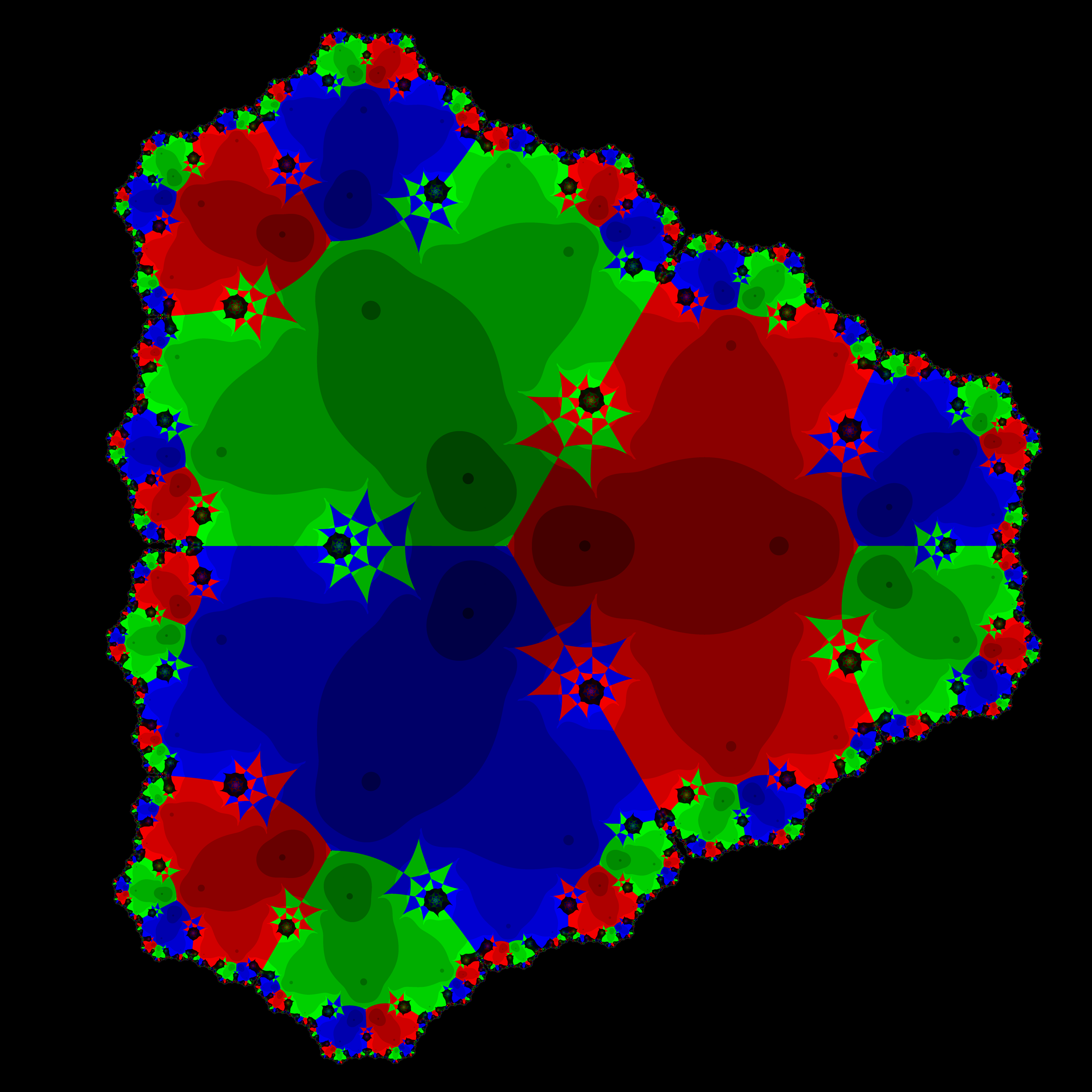
8. Adding poles to the standard case
The traditional Newton's Fractal uses the cubic map \(f(x)=z^3-1\), but any function can be used. This function is continuous on the entire complex plain. What happens when we introduce some poles? An interesting place to put the poles would be to mirror the roots of \(f\) across the imaginary axis. That is to say, for any root \(x+yi\) of \(f\) we add a pole at \(-x+yi\). The corresponding function is:
\[f=\frac{z^3-1}{z^3+1}\]
Note we add a bail out condition if \(z\) gets too big. I do this to speed things up because of the large number of points in the region that don't converge to a root. Normally I wouldn't do this for a Newton fractal rendering because it will cause us to fail to recognize some points converge – because orbits that converge can have points of very large modulus. The good news is that the final product is very similar with and without the bailout, but it runs an order of magnitude faster with the bailout.
#include "ramCanvas.hpp"

typedef mjr::ramCanvas3c8b rcT;    // The Ram Canvas type we will use

int main(void) {
  std::chrono::time_point<std::chrono::system_clock> startTime = std::chrono::system_clock::now();
  const int            MAXITR = 255;
  const int            COLMAG = 300;
  const int            CCLMAG = 300;
  const double         ZMAGMX = 1e10;
  const double         RELSIZ = 2.1;
  const double         XCENTR = 0.35;
  const double         YCENTR = 0.0;
  const double         ZROEPS = .0001;
  const int            IMGSIZ = 7680/1;
  const  double        r      = 1.0;
  std::complex<double> r1( 1.0,                        0.0);
  std::complex<double> r2(-0.5,  sin(2*std::numbers::pi/3));
  std::complex<double> r3(-0.5, -sin(2*std::numbers::pi/3));
  rcT                  theRamCanvas(IMGSIZ, IMGSIZ, XCENTR-RELSIZ, XCENTR+RELSIZ, YCENTR-RELSIZ, YCENTR+RELSIZ);

# pragma omp parallel for schedule(static,1)
  for(int y=0;y<theRamCanvas.getNumPixY();y++) {
#   pragma omp critical
    if ((y%(IMGSIZ/100))==0)
      std::cout << "line " << y << " of " << IMGSIZ << std::endl;
    for(int x=0;x<theRamCanvas.getNumPixX();x++) {
      std::complex<double> z = theRamCanvas.int2real(x, y);
      for(int count=0; count<MAXITR; count++) {
        if(std::abs(z) < 2) {
          if(std::abs(z-r1) <= ZROEPS) {
            theRamCanvas.drawPoint(x, y, rcT::colorType::csCCu0R::c(count*CCLMAG)); break;
          } else if(std::abs(z-r2) <= ZROEPS) {
            theRamCanvas.drawPoint(x, y, rcT::colorType::csCCu0G::c(count*CCLMAG)); break;
          } else if(std::abs(z-r3) <= ZROEPS) {
            theRamCanvas.drawPoint(x, y, rcT::colorType::csCCu0B::c(count*CCLMAG)); break;
          } else if(std::abs(z) <= ZROEPS) {
            break;
          }
        } else {
          if(std::abs(z) > ZMAGMX) {
            theRamCanvas.drawPoint(x, y, rcT::colorType::csCCu0W::c(count*COLMAG)); break;
            break;
          }
        }
        z = (-pow(z, 0.6e1) + (0.2e1 * r + 0.4e1) * pow(z, 0.3e1) + r) * pow(z, -0.2e1) / (r + 0.1e1) / 0.3e1;
      }
    }
  }
  theRamCanvas.writeTIFFfile("newton_3updown.tiff");
  std::chrono::duration<double> runTime = std::chrono::system_clock::now() - startTime;
  std::cout << "Total Runtime " << runTime.count() << " sec" << std::endl;
}
The above program will generate this picture:
9. Newton's Method applied to a 6th degree polynomial
The traditional Newton's Fractal uses the cubic map \(f(x)=z^3-1\), but any function can be used. For example, we can use
\[f(x)=z^6-1\]
The code is identical except for the equation and more cases (for each root):
#include "ramCanvas.hpp"

typedef mjr::ramCanvas3c8b rcT;    // The Ram Canvas type we will use

int main(void) {
  std::chrono::time_point<std::chrono::system_clock> startTime = std::chrono::system_clock::now();
  constexpr  int              COLMAG = 25;
  constexpr rcT::coordIntType IMGSIZ = 7680;
  constexpr int               MAXITR = 155;
  constexpr rcT::coordFltType ZROEPS = 1.0e-5;
  constexpr rcT::cplxFltType  r1( 1.0,  0.0);
  constexpr rcT::cplxFltType  r2(-0.5,  std::sin(2.0*std::numbers::pi/3.0));
  constexpr rcT::cplxFltType  r3(-0.5, -std::sin(2.0*std::numbers::pi/3.0));
  constexpr rcT::cplxFltType  r4(-1.0,  0.0);
  constexpr rcT::cplxFltType  r5( 0.5,  std::sin(2.0*std::numbers::pi/3.0));
  constexpr rcT::cplxFltType  r6( 0.5, -std::sin(2.0*std::numbers::pi/3.0));

  rcT theRamCanvas(IMGSIZ, IMGSIZ, -1.20, 1.20, -1.20, 1.20);

# pragma omp parallel for schedule(static,1)
  for(rcT::coordIntType y=0;y<theRamCanvas.getNumPixY();y++) {
    for(rcT::coordIntType x=0;x<theRamCanvas.getNumPixX();x++) {
      rcT::cplxFltType z = theRamCanvas.int2real(x, y);
      for(int count=0; count<MAXITR; count++) {
        if(std::abs(z-r1) <= ZROEPS) {
          theRamCanvas.drawPoint(x, y, rcT::colorType::csCCu0R::c(255-count*COLMAG)); break;
        } else if(std::abs(z-r2) <= ZROEPS) {
          theRamCanvas.drawPoint(x, y, rcT::colorType::csCCu0G::c(255-count*COLMAG)); break;
        } else if(std::abs(z-r3) <= ZROEPS) {
          theRamCanvas.drawPoint(x, y, rcT::colorType::csCCu0B::c(255-count*COLMAG)); break;
        } else if(std::abs(z-r4) <= ZROEPS) {
          theRamCanvas.drawPoint(x, y, rcT::colorType::csCCu0M::c(255-count*COLMAG)); break;
        } else if(std::abs(z-r5) <= ZROEPS) {
          theRamCanvas.drawPoint(x, y, rcT::colorType::csCCu0C::c(255-count*COLMAG)); break;
        } else if(std::abs(z-r6) <= ZROEPS) {
          theRamCanvas.drawPoint(x, y, rcT::colorType::csCCu0Y::c(255-count*COLMAG)); break;
        } else if(std::abs(z) <= ZROEPS) {
          break;
        }
        rcT::cplxFltType tmp = pow(z, 5);
        z = z-(tmp*z-1.0)/(6.0*tmp);
      }
    }
  }
  /* The biggest reason homogeneous transforms are in the library is to support color scale correction.  */
  theRamCanvas.applyHomoPixTfrm(&rcT::colorType::tfrmLinearGreyLevelScale, 255.0 / 155, 0.0);
  theRamCanvas.autoHistStrech();
  theRamCanvas.writeTIFFfile("newton_z6.tiff");
  std::chrono::duration<double> runTime = std::chrono::system_clock::now() - startTime;
  std::cout << "Total Runtime " << runTime.count() << " sec" << std::endl;
}
The above program will generate this picture:
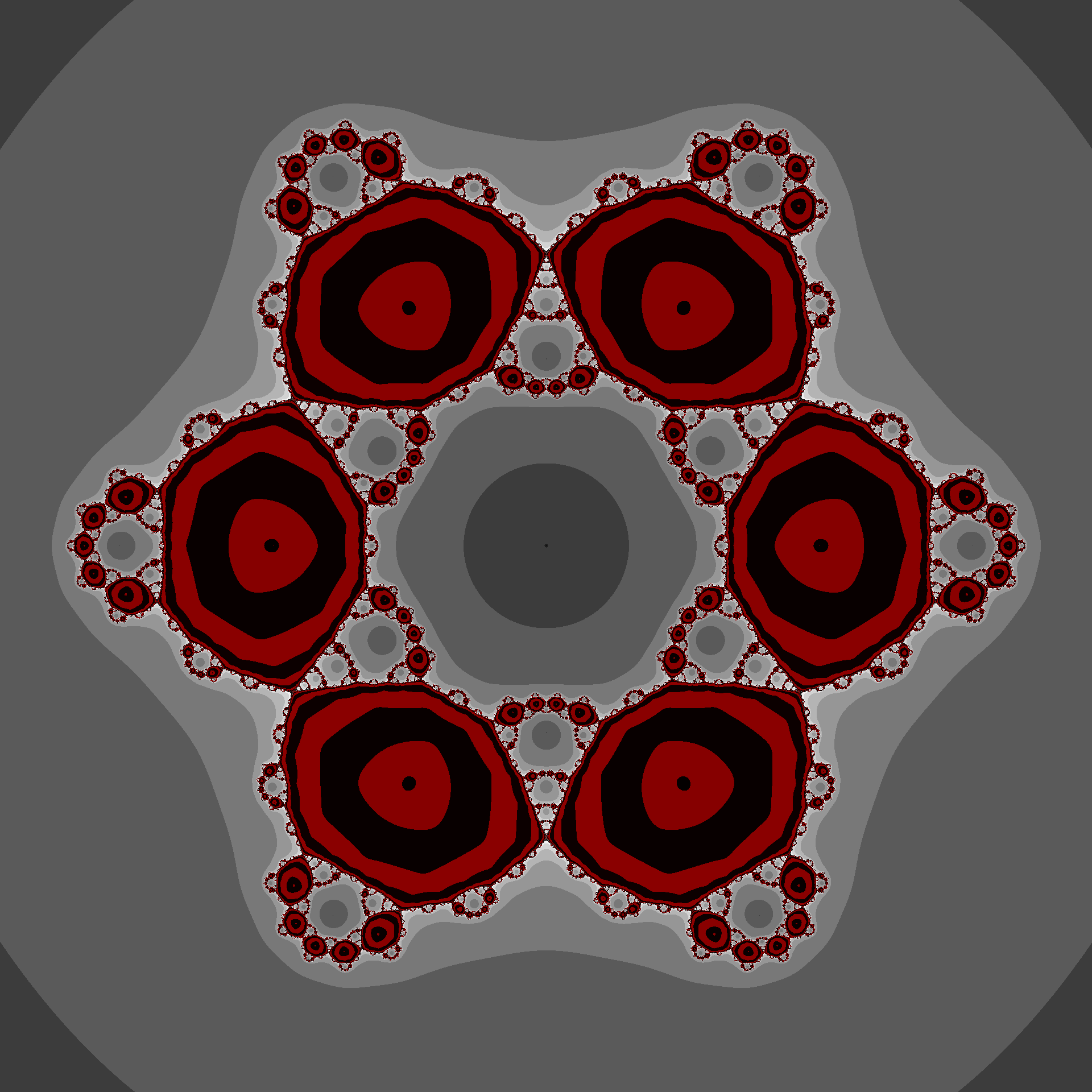
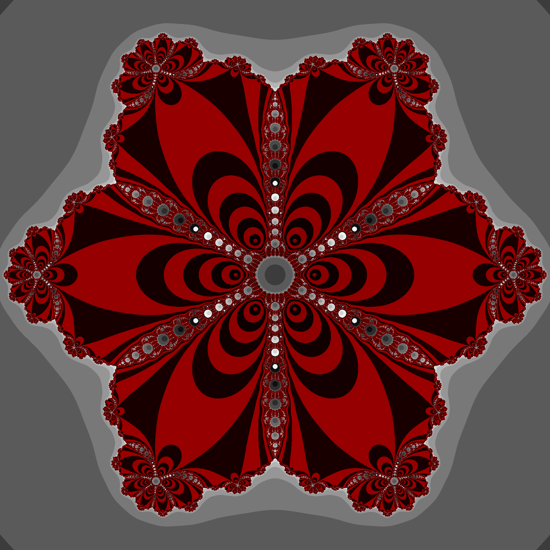
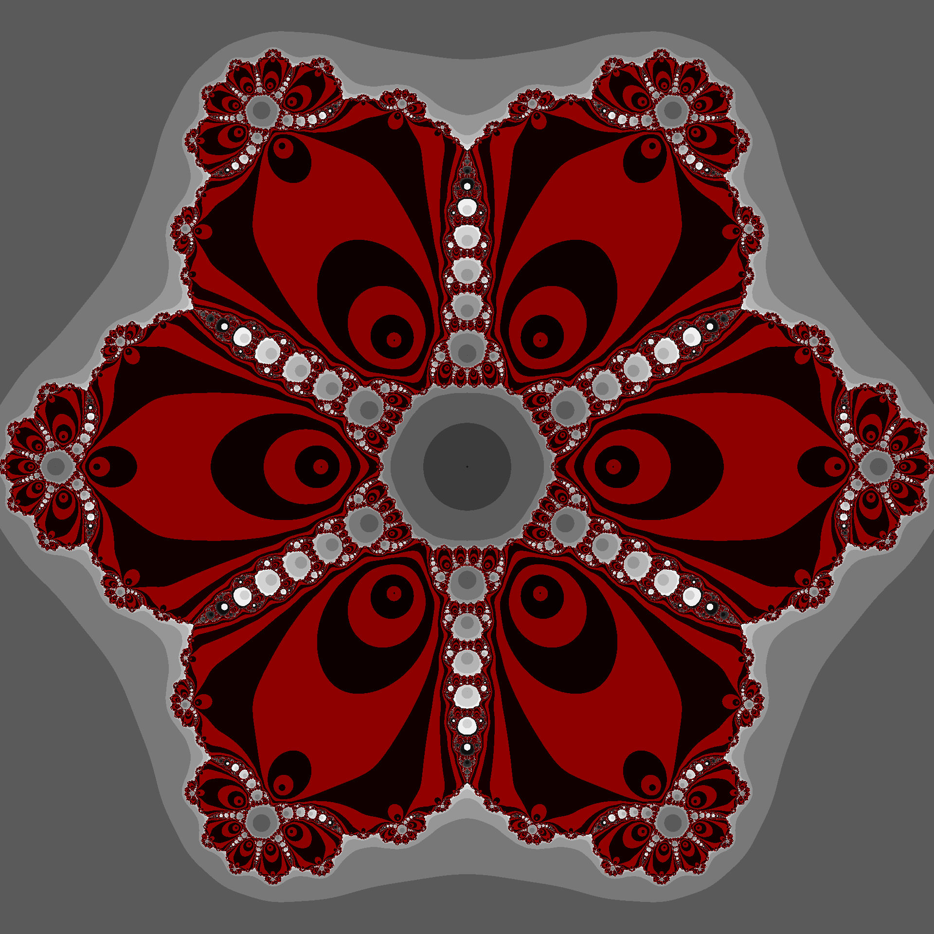
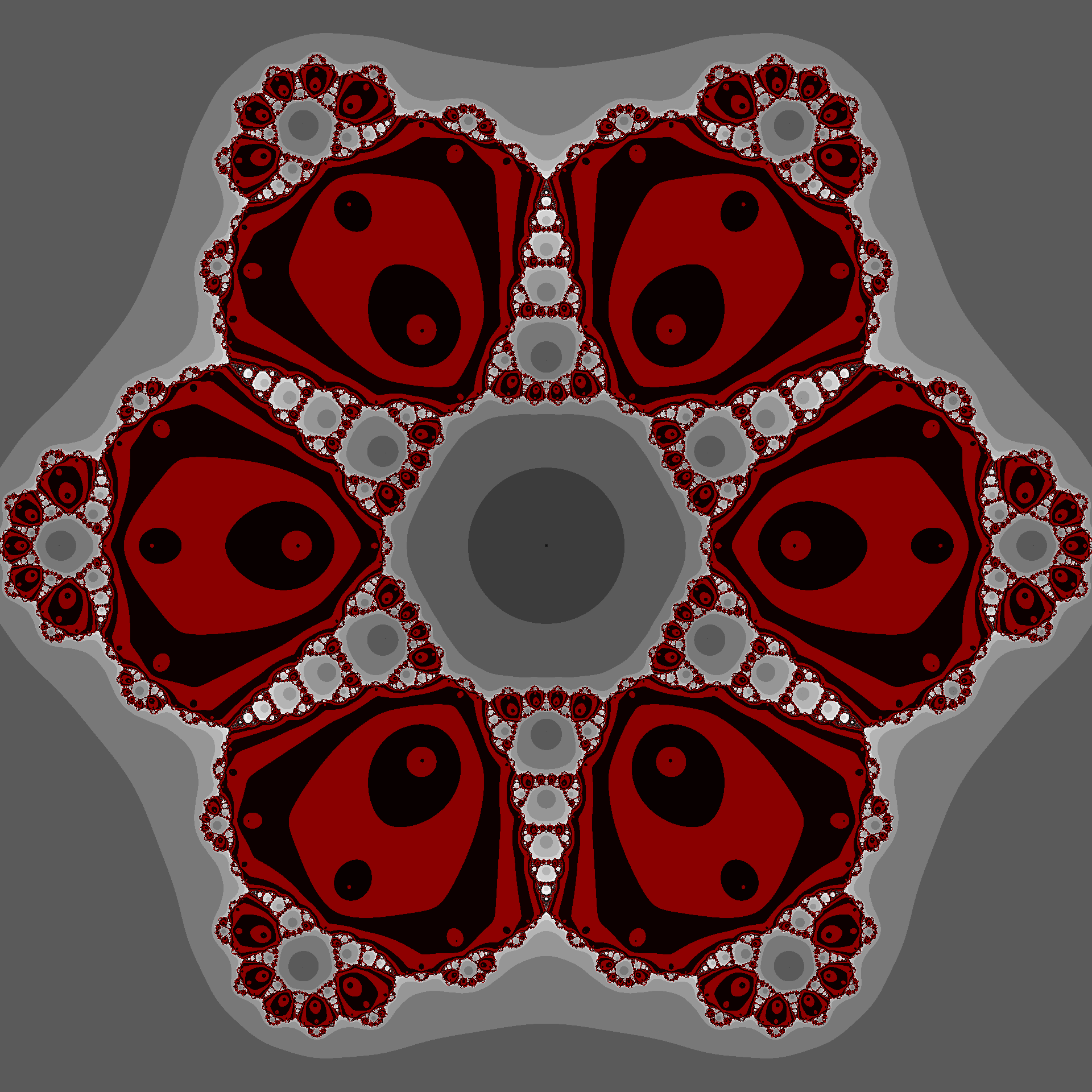
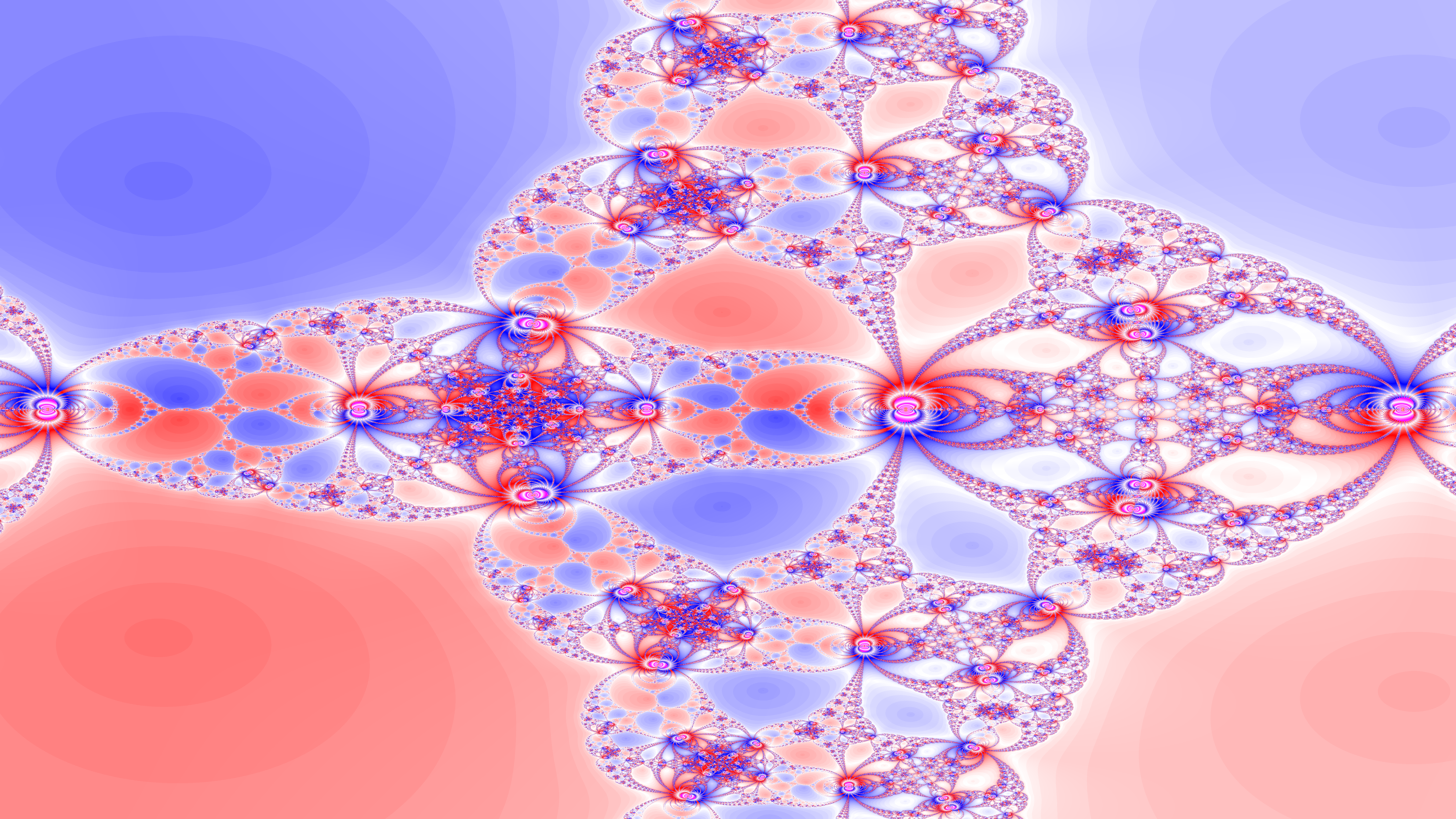
10. Adding poles to the 6th degree case
Now we combine the previous two sections and add poles to the 6th degree case. We observed a serious change in behavior for Newton's method in the degree 3 case with the poles situated on arguments midway between the roots. Just how sensitive is Newton's method to poles? We can explore this question by placing poles at different places, and observing the changes. Just for fun lets place our poles on a ring around the axis, and rotate them – like 6 planets sharing the same orbit of the sun. We will be considering the impact when the orbit is of diameter \(\frac{1}{100}\), \(\frac{3}{2}\), \(10\), \(100\), and \(10,000\). Why these choices? The first, \(\frac{1}{100}\), is interesting because all the singularities are so close together – the roots are 100 radii distant! The second, \(\frac{3}{2}\), is interesting because it places the poles on a ring just outside the roots. The last three are interesting because they move the ring out further and further.
#include "ramCanvas.hpp"

typedef mjr::ramCanvas3c8b rcT;    // The Ram Canvas type we will use

int main(void) {
  std::chrono::time_point<std::chrono::system_clock> startTime = std::chrono::system_clock::now();
  const int                  MAXITR = 255;
  const int                  CCLMAG = 130;
  const int                  DCLMAG = 30;
  const int                  NUMFRM = 4*8;
  const double               ZMAGMX = 1e10;
  const double               RELSIZ = 7.0;
  const double               XCENTR = 0.0;
  const double               YCENTR = 0.0;
  const double               ZROEPS = .0001;
  const int                  IMGSIZ = 7680/16;
  const std::complex<double> r1( 1.0,                             0.0);
  const std::complex<double> r2(-0.5,  std::sin(2*std::numbers::pi/3));
  const std::complex<double> r3(-0.5, -std::sin(2*std::numbers::pi/3));

# pragma omp parallel for schedule(static,1)
  for(int frame=0; frame<NUMFRM; frame++) {
#   pragma omp critical
    std::cout << "frame " << (frame+1) << " of " << NUMFRM << std::endl;
    rcT theRamCanvas(IMGSIZ, IMGSIZ, XCENTR-RELSIZ, XCENTR+RELSIZ, YCENTR-RELSIZ, YCENTR+RELSIZ);
    double angle = 2.0*std::numbers::pi/6.0/NUMFRM*frame;
    std::complex<double> a(std::cos(angle), std::sin(angle));
    double b = 1e-2;
    for(int y=0;y<theRamCanvas.getNumPixY();y++) {
      for(int x=0;x<theRamCanvas.getNumPixX();x++) {
        std::complex<double> z  = theRamCanvas.int2real(x, y);
        std::complex<double> zL = z + 100.0;
        for(int count=0; count<MAXITR; count++) {
          if(std::abs(z-zL) <= ZROEPS) {
            theRamCanvas.drawPoint(x, y, rcT::colorType::csCCu0R::c(count*CCLMAG)); break;
          } else if(std::abs(z) <= ZROEPS) {
            break;
          } else if(std::abs(z) > ZMAGMX) {
            theRamCanvas.drawPoint(x, y, rcT::colorType::csCCu0W::c(count*DCLMAG)); break;
            break;
          }
          zL = z;
          if (b<1e11)
            z = (-pow(a, 6.0) * pow(z, 12.0) + (7.0 * pow(a, 6.0) + (5.0 * b)) * pow(z, 6.0) + b) /
                pow(z, 5.0) / (pow(a, 6.0) + b) / 6.0;
          else
            z = (5.0 * pow(z, 6.0) + 1.0) / pow(z, 5.0) / 6.0;
        }
      }
    }
    theRamCanvas.writeTIFFfile("newton_roter_" + mjr::fmtInt(frame, 3, '0') + ".tiff");
  }
  std::chrono::duration<double> runTime = std::chrono::system_clock::now() - startTime;
  std::cout << "Total Runtime " << runTime.count() << " sec" << std::endl;
}
The above program can generate the following movies:
 |
 |
| \(\frac{1}{100}\) case | \(\frac{3}{2}\) case |
 |
 |
 |
| \(R=10,000\) case | \(R=100\) case | \(R=10\) case |
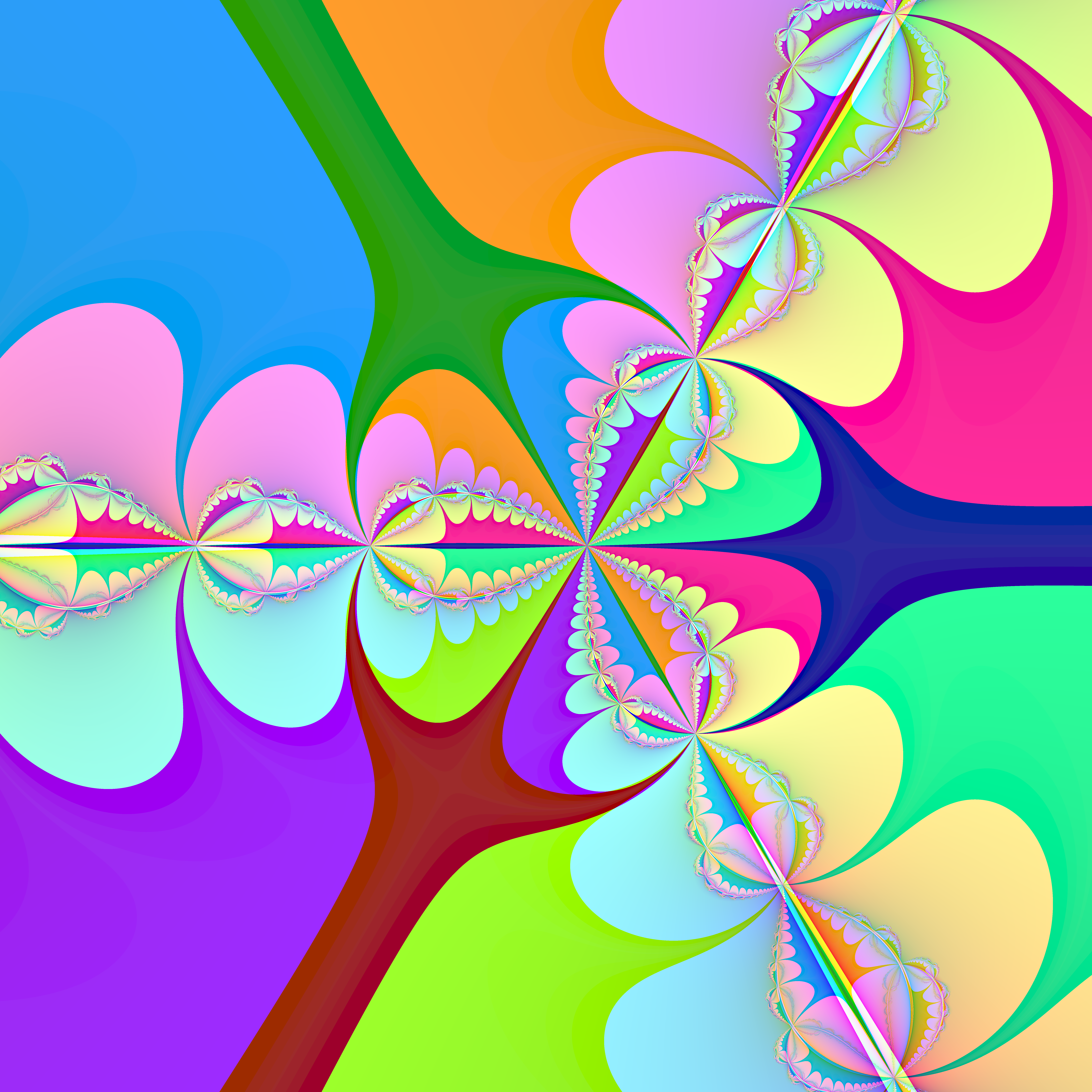
11. Newton's Method applied to non-polynomials
Of course we are not limited to applying Newton's method to polynomials. That said many complex functions have infinitely many roots, and thus it's impossible to shade our fractal in a distinct way for each root. So for this program I have decided to have the color hue indicate the following:
- Magenta for regions that didn't converge
- Blues for convergence to roots in the upper half plane
- Reds for convergence to roots in the lower half plane
- Black if the iterates become very large
- Cyan for division by zero
Note the code has several commented out sections with interesting alternative functions and plot ranges.
#include "ramCanvas.hpp"

typedef mjr::ramCanvas3c8b rcT;    // The Ram Canvas type we will use

/** Enum identifying why iteration stopped */
enum class whyStopNH { DIVZERO,   //!< Divide by zero (zeroTol)
                       TOOBIG,    //!< Iterate got too big (> escapeMod)
                       CONVERGEU, //!< Converged in the upper half plane
                       CONVERGEL, //!< Converged in the lower half plane
                       TOOLONG    //!< Too many iterations (> MaxCount)
                     };

int main(void) {
  std::chrono::time_point<std::chrono::system_clock> startTime = std::chrono::system_clock::now();
  constexpr rcT::coordIntType IMXSIZ    = 7680;
  constexpr rcT::coordIntType IMYSIZ    = 4320;
  constexpr double            MAXZ      = -32.0;
  constexpr int               MAXITR    = 64;
  constexpr double            ZROEPS    = 0.0001;
  constexpr int               numToKeep = 5;
  whyStopNH                   why;
  rcT::colorType              aColor(255, 255, 255);
  // rcT                       theRamCanvas(IMXSIZ, IMYSIZ, 4.0, 8.0, -2.0, 2.0);
  // rcT                       theRamCanvas(IMXSIZ, IMYSIZ, -0.16, 0.36, -0.22, 0.23);
  // rcT                       theRamCanvas(IMXSIZ, IMYSIZ, -0.42, 0.42, -0.2, 0.2);
  // rcT                       theRamCanvas(IMXSIZ, IMYSIZ, -4.72, -0.5, -1.0, 1.0);
  // rcT                       theRamCanvas(IMXSIZ, IMYSIZ, -3.0, 3.0, -3.0, 3.0);
  rcT                         theRamCanvas(IMXSIZ, IMXSIZ, 0.6, 1.1, -0.4, 0.4); // this one is square!

# pragma omp parallel for schedule(static,1)
  for(int y=0;y<theRamCanvas.getNumPixY();y++) {
#   pragma omp critical
    std::cout << "Line: " << y << " of " << theRamCanvas.getNumPixY() << std::endl;
    for(int x=0;x<theRamCanvas.getNumPixX();x++) {
      std::complex<double> z = theRamCanvas.int2real(x, y);

      std::vector<std::complex<double>> lastZs(numToKeep);
      rcT::csIntType count = 0;
      double maxMod = 0.0;
      while(1) {
        if (count >= MAXITR) {
          why = whyStopNH::TOOLONG;
          break;
        }
        // std::complex<double> cz = ((-2.0*sin(2.0*z))-sin(z)+1.0);
        // std::complex<double> cz = (exp(z)-1.0);
        // std::complex<double> cz = sin(z);
        // std::complex<double> cz = cos(z);
        // std::complex<double> cz = ((2.0*z*cos(z)-z*z*sin(z))*cos(z*z*cos(z)));
        std::complex<double> cz = ((cos(z)-z*sin(z))*cos(z*cos(z)));
        if(std::abs(cz) < ZROEPS) {
          why = whyStopNH::DIVZERO;
          break;
        }
        // z = z-(cos(2.0*z)+cos(z)+z)/cz;
        // z = z-(exp(z)-z)/cz;
        // z = z+cos(z)/cz;
        // z = z-(sin(z)-0.9)/cz;
        // z=z-sin(z*z*cos(z))/cz;
        z=z-sin(z*cos(z))/cz;
        double modz = std::abs(z);
        lastZs[count%numToKeep] = z;
        if(modz>maxMod) {
          maxMod = modz;
        }
        if(count >= numToKeep) {  // Criteria for convergeance:  Last numToKeep z values must be within ZROEPS of each other.
          bool allEqual = true;
          for(int i=1; i<numToKeep; i++)
            if(std::abs(lastZs[0]-lastZs[i])>ZROEPS) {
              allEqual = false;
              break;
            }
          if(allEqual) {
            if(std::imag(z) > 0) {
            //if(std::real(z) > 0) {
              why = whyStopNH::CONVERGEU;
            } else {
              why = whyStopNH::CONVERGEL;
            }
            break;
          }
        }
        if((MAXZ>0) && (modz>MAXZ)) {
          why = whyStopNH::TOOBIG;
          break;
        }
        count++;
      }

      rcT::csIntType ccol = (2*4*count);
      rcT::csIntType mcol = ((rcT::csIntType)(2*8*maxMod));
      switch(why) {
        case whyStopNH::TOOLONG   : theRamCanvas.drawPoint(x, y, rcT::colorType::csCCwicM::c(mcol));      break;
        case whyStopNH::CONVERGEU : theRamCanvas.drawPoint(x, y, rcT::colorType::csCCwicB::c(mcol+ccol)); break;
        case whyStopNH::CONVERGEL : theRamCanvas.drawPoint(x, y, rcT::colorType::csCCwicR::c(mcol+ccol)); break;
        case whyStopNH::TOOBIG    : theRamCanvas.drawPoint(x, y, rcT::colorType("black"));                break;
        case whyStopNH::DIVZERO   : theRamCanvas.drawPoint(x, y, rcT::colorType::csCCwicC::c(mcol+ccol)); break;
      }
    }
  }
  theRamCanvas.writeTIFFfile("newton_half.tiff");
  std::chrono::duration<double> runTime = std::chrono::system_clock::now() - startTime;
  std::cout << "Total Runtime " << runTime.count() << " sec" << std::endl;
}
The above program will generate this picture:
Several alternative functions and plot ranges are commented out in the code. These commented out sections generate the following:
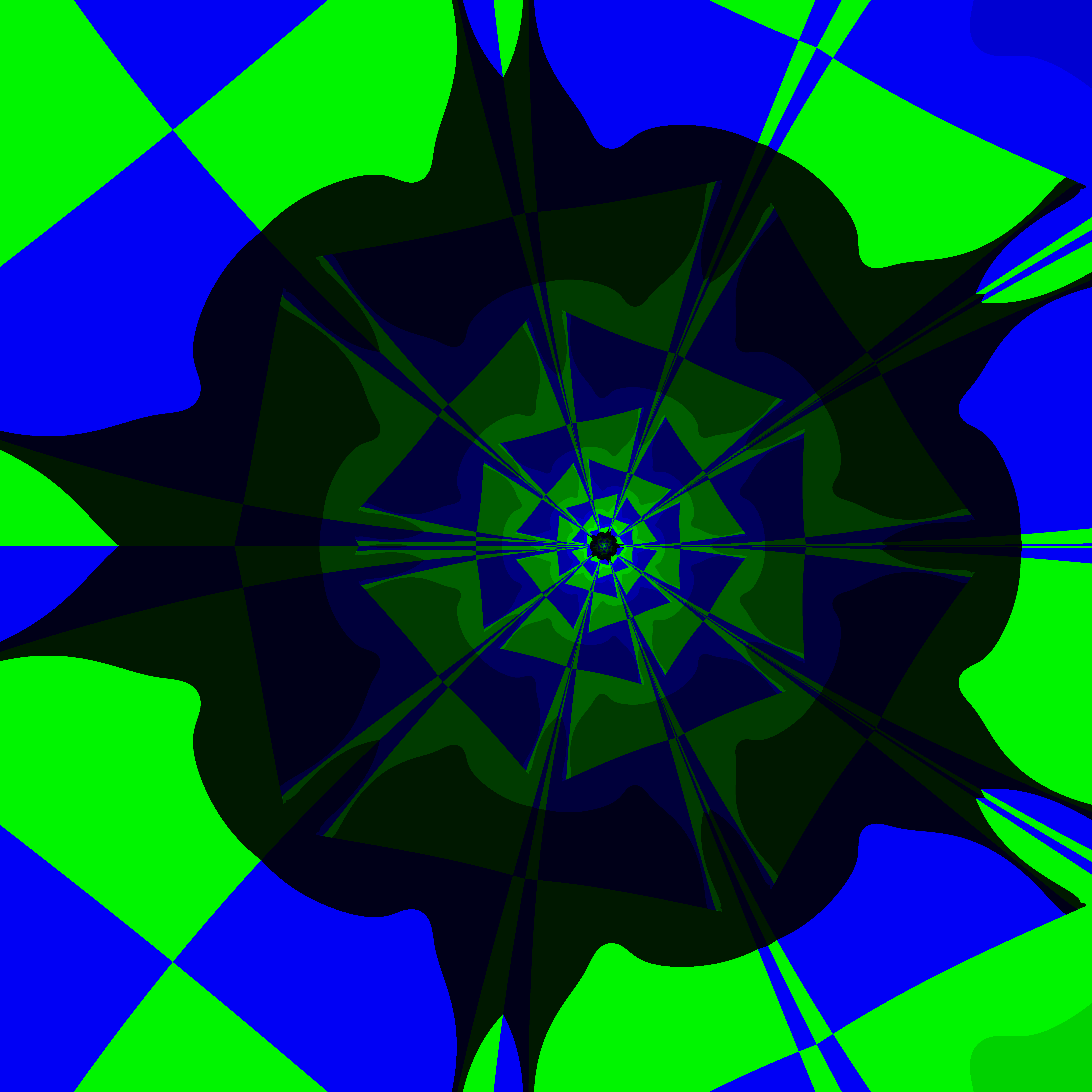
12. Modified Newton's Fractals
A very slight change to Newton's method is frequently used to generate different fractals. The normal Newton iteration is defined by the following equation:
\[z_{n+1}=z_n-\frac{f(z_n)}{f'(z_n)}\]
We simply add a factor to the equation thus modifying the delta at each step like so:
\[z_{n+1}=z_n-\alpha\frac{f(z_n)}{f'(z_n)}\]
By varying the value for alpha, very different fractals are generated. Here is some code:
#include "ramCanvas.hpp"

typedef mjr::ramCanvas3c8b rcT;    // The Ram Canvas type we will use

int main(void) {
  std::chrono::time_point<std::chrono::system_clock> startTime = std::chrono::system_clock::now();
  int                  MAXITR = 255;
  double               ZROEPS = .0001;
  const int            IMGSIZ = 7680;
  std::complex<double> r1( 1.0,                        0.0);
  std::complex<double> r2(-0.5,  sin(2*std::numbers::pi/3));
  std::complex<double> r3(-0.5, -sin(2*std::numbers::pi/3));
  rcT                  theRamCanvas(IMGSIZ, IMGSIZ, -1.3, 1.3, -1.3, 1.3); // -0.9, -0.7, -0.1, 0.1
  // std::complex<double> alpha( 1.0,  0.0);
  // std::complex<double> alpha( 2.0,  0.0);
  // std::complex<double> alpha( 2.2,  0.0);
  // std::complex<double> alpha( 2.5,  0.0);
  // std::complex<double> alpha( 2.9,  0.0);
  // std::complex<double> alpha(-0.5,  0.0);
  // std::complex<double> alpha(-0.1, -0.1);
  // std::complex<double> alpha(-0.1,  0.0);
  // std::complex<double> alpha(-0.1,  0.1);
  // std::complex<double> alpha(-0.1,  0.2);
  // std::complex<double> alpha(-0.1,  1.5);
  // std::complex<double> alpha(0.4,  0.5);
  std::complex<double> alpha( 1.1,  0.75);

# pragma omp parallel for schedule(static,1)
  for(int y=0;y<theRamCanvas.getNumPixY();y++) {
    if ((y%10)==0)
#     pragma omp critical
      std::cout << "Line: " << y << " of " << theRamCanvas.getNumPixY() << std::endl;
    for(int x=0;x<theRamCanvas.getNumPixX();x++) {
      std::complex<double> z = theRamCanvas.int2real(x, y);
      for(int count=0; count<MAXITR; count++) {
        if(std::abs(z) <= ZROEPS)
          break;
        z = z-alpha*(z*z*z-1.0)/(z*z*3.0);
      }
      theRamCanvas.drawPoint(x, y, rcT::colorType::csCColdeRainbow::c(1.0-std::arg(z)/std::numbers::pi));
    }
  }
  theRamCanvas.writeTIFFfile("newton_modified_C.tiff");
  std::chrono::duration<double> runTime = std::chrono::system_clock::now() - startTime;
  std::cout << "Total Runtime " << runTime.count() << " sec" << std::endl;
}
The above program will generate this picture:
The commented out values for alpha produce the following:

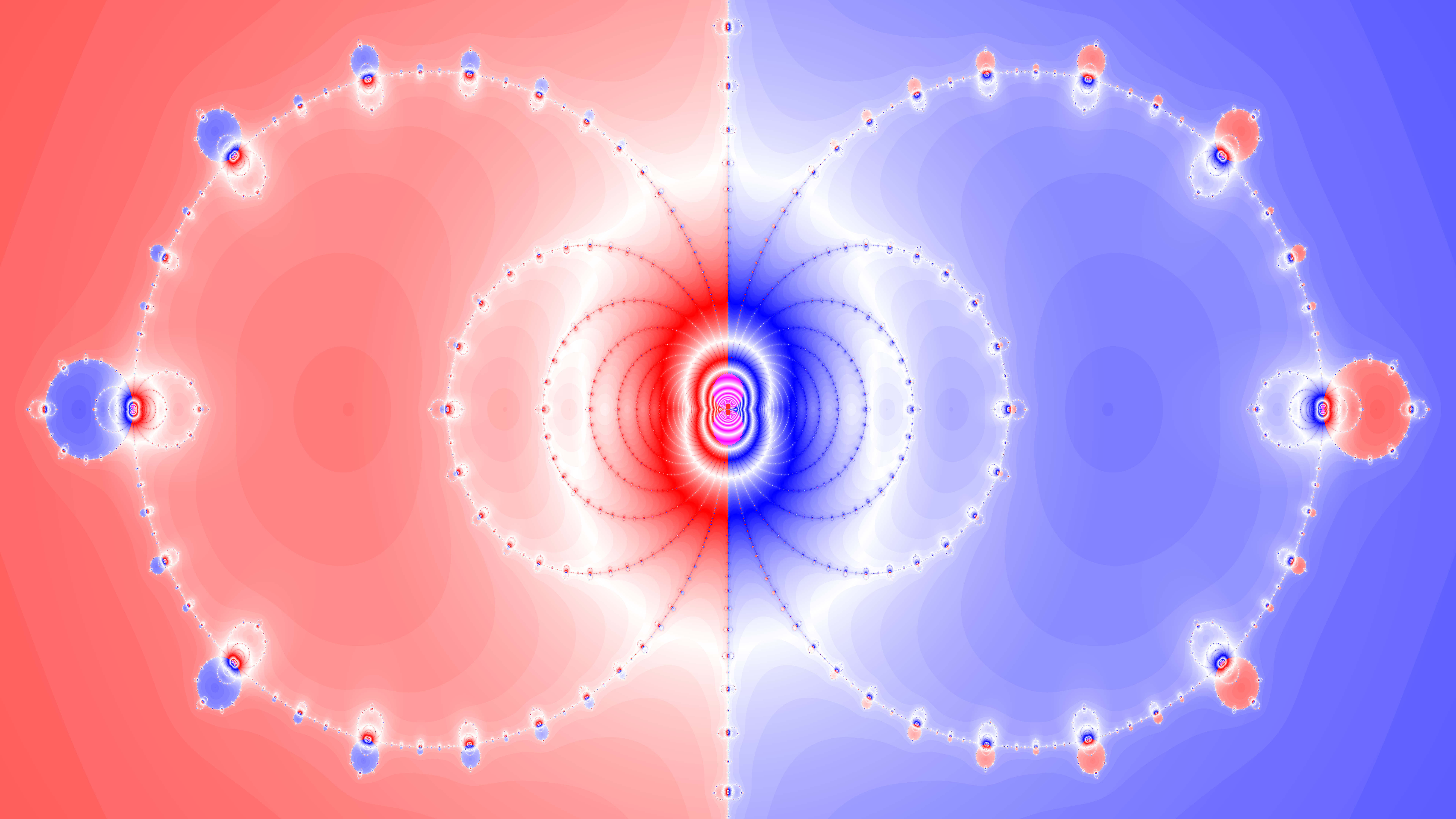
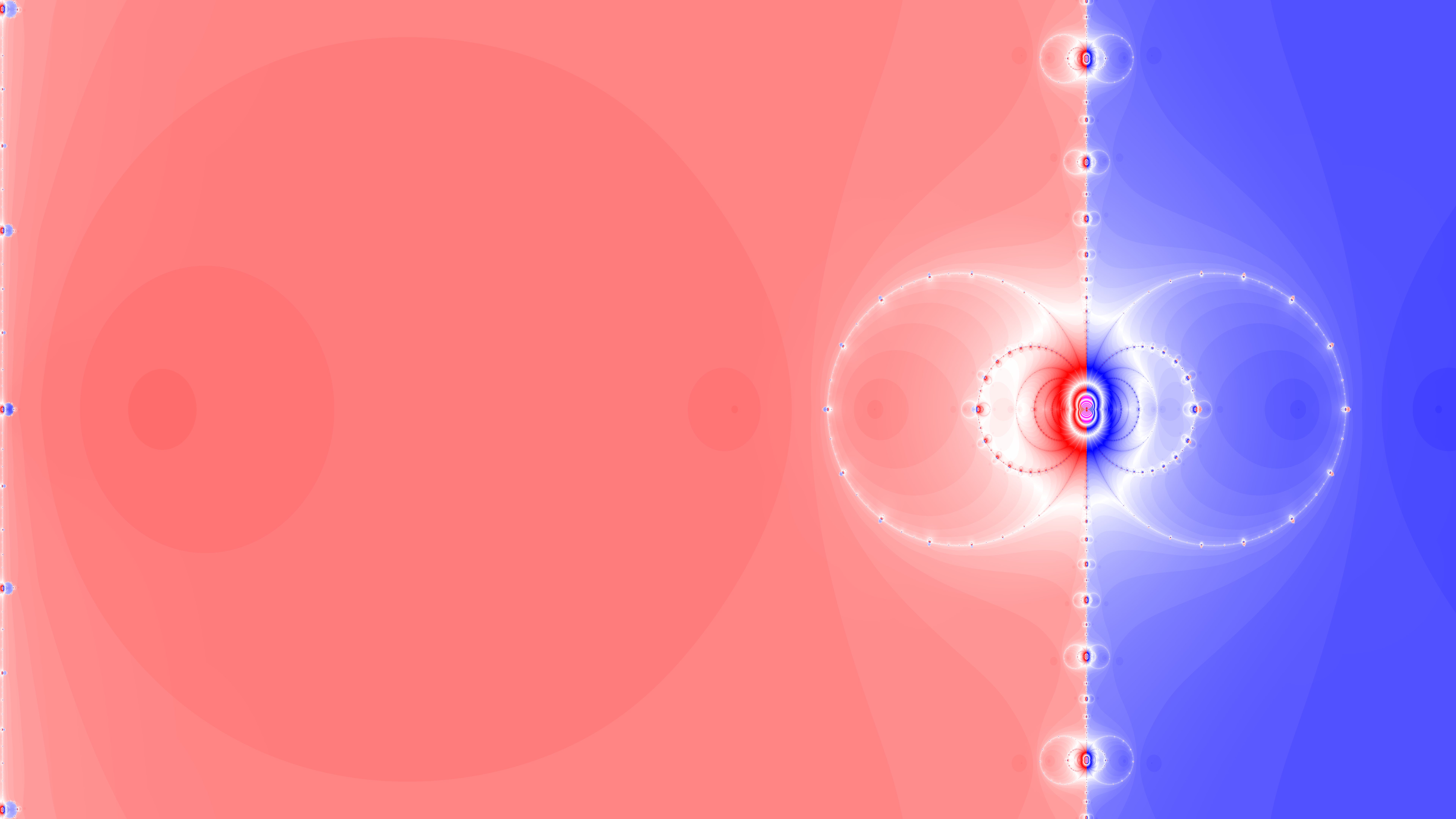
13. Moving beyond Newton: Laguerre's Method
Not all iterative methods are chaotic. Laguerre's method, for example, seems almost magically stable after playing around with Newton's method. If we return to our original objective function, \(f(x)=z^3-1\), and plot the regions of convergence for Laguerre's method we get a pretty boring image!
Here is some code:
#include "ramCanvas.hpp"

int main(void) {
  std::chrono::time_point<std::chrono::system_clock> startTime = std::chrono::system_clock::now();
  const int            MAXITR = 255;
  const double         ZROEPS = 0.0001;
  const int            IMGSIZ = 7680/1;
  std::complex<double> r1( 1.0,                        0.0);
  std::complex<double> r2(-0.5,  sin(2*std::numbers::pi/3));
  std::complex<double> r3(-0.5, -sin(2*std::numbers::pi/3));
  mjr::ramCanvas3c8b   theRamCanvas(IMGSIZ, IMGSIZ, -2.0, 2, -2, 2); // -0.9, -0.7, -0.1, 0.1

# pragma omp parallel for schedule(static,1)
  for(int y=0;y<theRamCanvas.getNumPixY();y++) {
    for(int x=0;x<theRamCanvas.getNumPixX();x++) {
      std::complex<double> z = theRamCanvas.int2real(x, y);
      for(int count=0; count<MAXITR; count++) {
        if(std::abs(z-r1) <= ZROEPS) {
          theRamCanvas.drawPoint(x, y, "red"); break;
        } else if(std::abs(z-r2) <= ZROEPS) {
          theRamCanvas.drawPoint(x, y, "green"); break;
        } else if(std::abs(z-r3) <= ZROEPS) {
          theRamCanvas.drawPoint(x, y, "blue"); break;
        } else if(std::abs(z) <= ZROEPS) {
          break;
        }
        std::complex<double> G = 3.0 * z * z / (pow(z, 3.0) - 1.0);
        std::complex<double> ABR = 6.0 * sqrt(z / pow(pow(z, 3.0) - 1.0, 2.0));
        std::complex<double> ABP = G + ABR;
        std::complex<double> ABN = G - ABR;
        std::complex<double> AB = (std::abs(ABP) > std::abs(ABN) ? ABP : ABN);
        z = z - 3.0 / AB;
      }
    }
  }
  theRamCanvas.writeTIFFfile("laguerre_simple.tiff");
  std::chrono::duration<double> runTime = std::chrono::system_clock::now() - startTime;
  std::cout << "Total Runtime " << runTime.count() << " sec" << std::endl;
}
The above program will generate this picture:

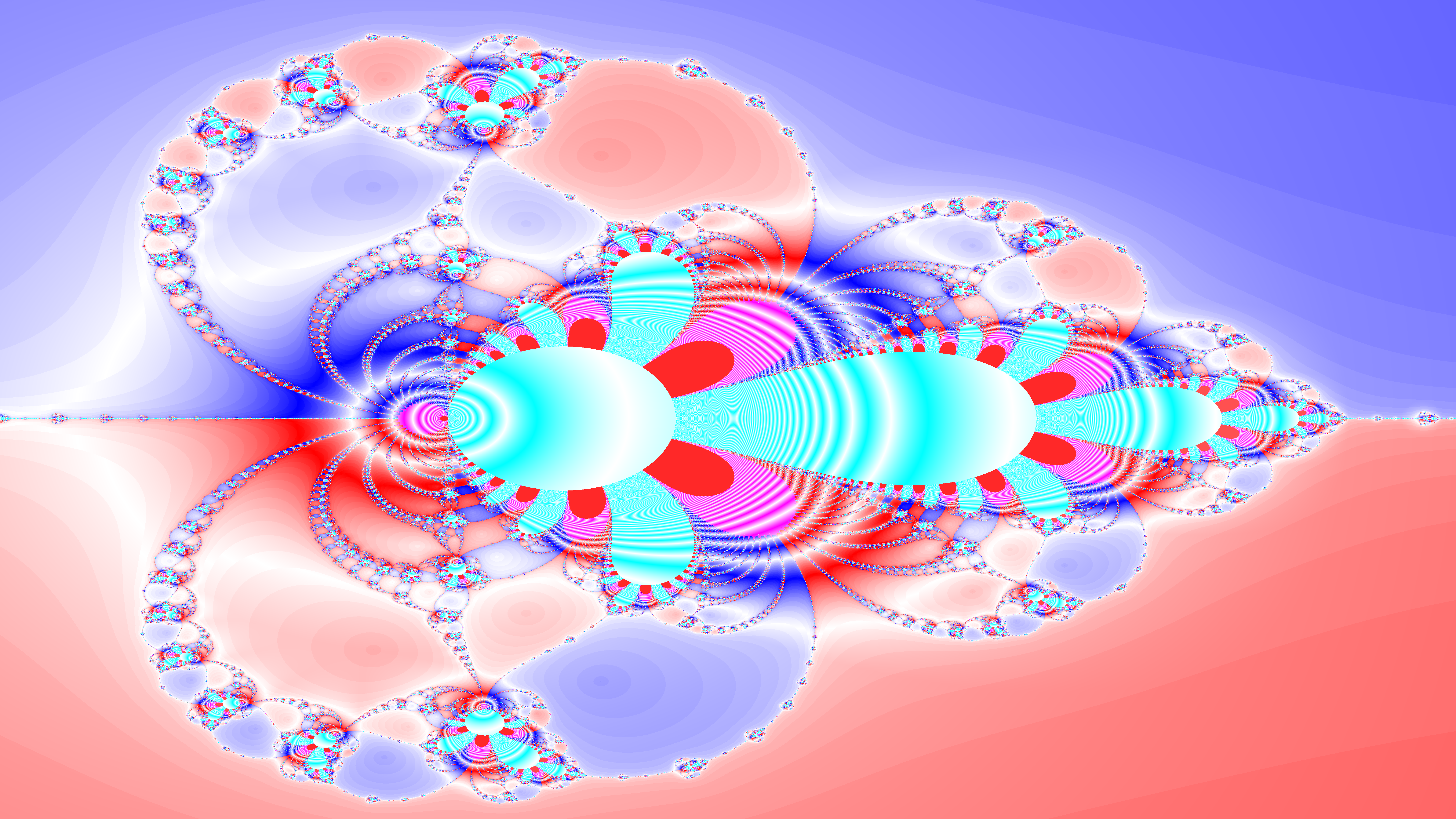
14. Laguerre's method with poles
From the previous section one might get the impression that Laguerre is boring and not very useful for fractals! Not the case. We just need to abuse the method a bit. Laguerre's method is only magically delicious for polynomial objective functions! If we add some poles like we did above with Newton's method, then Laguerre's method can produce some very interesting fractals too!
Here is some code:
#include "ramCanvas.hpp"

int main(void) {
  std::chrono::time_point<std::chrono::system_clock> startTime = std::chrono::system_clock::now();
  const int            MAXITR = 255;
  const int            CCLMAG = 35;
  const double         ZMAGMX = 1e10;
  const double         YCENTR = 0.0;
  const double         ZROEPS = .0001;
  const int            IMGSIZ = 7680/1;
  const double         RELSIZ =  4.0; //  0.55;  14.5;  4.0;   0.15;
  const double         XCENTR =  0.5; //  -4.7;   1.5;  0.5;  -0.20;
  const double         r      =  1.0; // 100.0; 100.0;  1.0;  0.001;
  std::complex<double> r1( 1.0,                        0.0);
  std::complex<double> r2(-0.5,  sin(2*std::numbers::pi/3));
  std::complex<double> r3(-0.5, -sin(2*std::numbers::pi/3));
  mjr::ramCanvas3c8b theRamCanvas(IMGSIZ, IMGSIZ, XCENTR-RELSIZ, XCENTR+RELSIZ, YCENTR-RELSIZ, YCENTR+RELSIZ);

# pragma omp parallel for schedule(static,1)
  for(int y=0;y<theRamCanvas.getNumPixY();y++) {
#   pragma omp critical
    if ((y%(IMGSIZ/100))==0)
      std::cout << "line " << y << " of " << IMGSIZ << std::endl;
    for(int x=0;x<theRamCanvas.getNumPixX();x++) {
      std::complex<double> z = theRamCanvas.int2real(x, y);
      for(int count=0; count<MAXITR; count++) {
        if(std::abs(z-r1) <= ZROEPS) {
          theRamCanvas.drawPoint(x, y, mjr::ramCanvas3c8b::colorType::csCCu0R::c(count*CCLMAG)); break;
        } else if(std::abs(z-r2) <= ZROEPS) {
          theRamCanvas.drawPoint(x, y, mjr::ramCanvas3c8b::colorType::csCCu0G::c(count*CCLMAG)); break;
        } else if(std::abs(z-r3) <= ZROEPS) {
          theRamCanvas.drawPoint(x, y, mjr::ramCanvas3c8b::colorType::csCCu0B::c(count*CCLMAG)); break;
        } else if(std::abs(z) <= ZROEPS) {
          break;
        } else if(std::abs(z) > ZMAGMX) {
          break;
        }
        std::complex<double> G = 3.0 * z * z * (r + 1.0) / (pow(z, 3.0) - 1.0) / (pow(z, 3.0) + r);
        std::complex<double> ABR = 6.0 * sqrt((r + 1.0) * (2.0 * pow(z, 6.0) - pow(z, 3.0) + r) * z /
                                              pow(pow(z, 3.0) - 1.0, 2.0) / pow(pow(z, 3.0) + r, 2.0));
        std::complex<double> ABP = G + ABR;
        std::complex<double> ABN = G - ABR;
        std::complex<double> AB = (std::abs(ABP) > std::abs(ABN) ? ABP : ABN);
        z = z - 3.0 / AB;
      }
    }
  }
  theRamCanvas.writeTIFFfile("laguerre_3updown.tiff");
  std::chrono::duration<double> runTime = std::chrono::system_clock::now() - startTime;
  std::cout << "Total Runtime " << runTime.count() << " sec" << std::endl;
}
The above program produced the following images:
 |
 |
|
| Case with \(R=\frac{1}{100}\) | Case with \(R=\frac{1}{100}\) Zoom to the ball near \(-1\) |
|
 |
||
| Case with \(R=10\) | ||
 |
 |
|
| Case with \(R=100\) | Case with \(R=100\) Zoom to the ball near \(-1\) |
15. Code
You can all the code included with MRaster.
16. References
Check out the fractals section of my reading list.