Mitch Richling: Peter de Jong Map (Attractor)
| Author: | Mitch Richling |
| Updated: | 2024-01-05 |
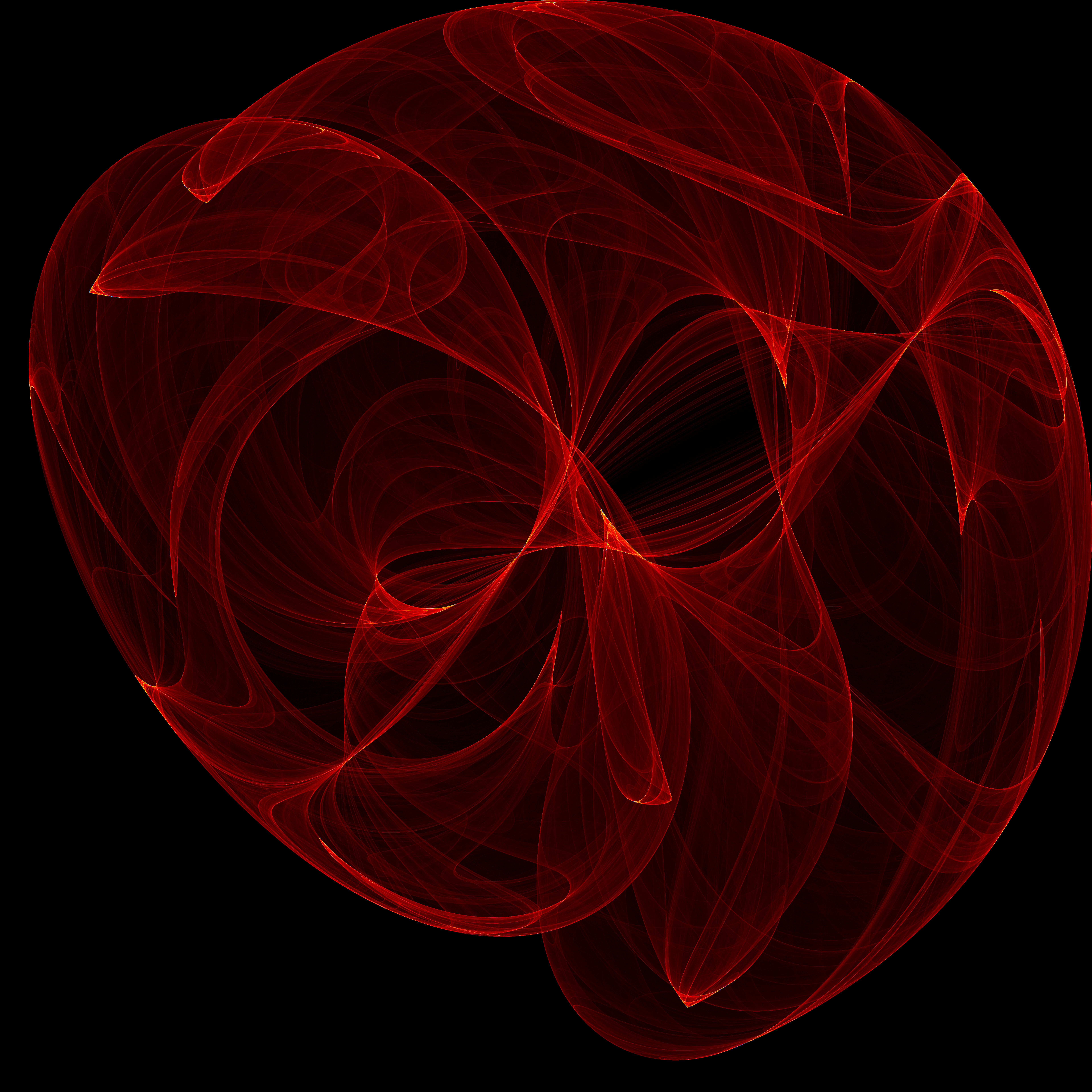
Table of Contents
1. Peter de Jong Map
The Peter de Jong map is an iterative system in two dimensions with four parameters (\(a\), \(b\), \(c\), and \(d\)). Each choice of parameter values will generate a different attractor. In addition to the four parameters, a set of initial conditions must also be specified. The defining equations are as follows:
\[\begin{align*} x_{n+1} & = \sin(a\cdot y_n) - \cos(b\cdot x_n) \\ y_{n+1} & = \sin(c\cdot x_n) - \cos(d\cdot y_n) \end{align*}\]
Various choices may be made for the initial conditions for the map. In the examples that follow, I have selected the following:
\[\begin{align*} x_0 & = 1 \\ y_0 & = 1 \\ \end{align*}\]
The global dynamics of a 2D iterative map can be partly illuminated by the probability density function, \(P(x,y)\), defined by the probability that some \((x_n, y_n)\) from the map will be in a neighborhood of \((x,y)\). While that sounds complicated, producing a visualization of this PDF is quite simple in practice – we simply visualize a histogram based on computed values of the map. The first step is to define a rectangular region of the plane over which we wish to visualize the PDF, and then define a set of discrete pixels over that region. Then we compute a few million, or billion, iterations of the map, and count the number of times we hit each pixel. That amounts to just a few lines of code in a sufficiently friendly language like Processing!
2. Code
Some code will make the above discussion clear:
#include "ramCanvas.hpp"

const int NPR = 18;

double params[NPR][9] = {
  /*        a         b         c         d          e          f          g         h     p */
  {  -1.68661, -1.99168,  1.71743, -1.64958,  0.299086, -1.293460, -0.054505, -1.73135, 2.00},   //  0 128822725
  {   1.50503, -1.44118, -1.23281,  1.78607,  1.709360,  1.794210,  1.893750, -1.38227, 2.10},   //  1 101379662
  {   1.81390,  1.30705, -1.94400, -1.48629,  0.242144,  0.075625, -0.480636, -0.18518, 1.75},   //  2 139794084
  {  -1.93281,  1.23020, -1.95848, -1.34156, -0.357486, -0.541028,  0.627957, -1.06337, 2.00},   //  3 118791871
  {   1.96082, -1.85272, -1.86495, -1.58137, -0.545130, -1.883680, -0.839783, -1.95953, 2.00},   //  4 102197049
  {   1.89361, -1.81593, -1.28357,  1.75597, -1.109410, -1.820460, -0.068557,  1.12429, 2.00},   //  5 107124786
  {  -1.76096, -1.68857, -1.33290,  1.98759, -1.104940,  1.947970, -1.414330,  1.31909, 2.00},   //  6  85670760
  {  -1.80149, -1.95335,  1.89633,  1.41626, -1.047470,  0.446659, -0.148925, -1.66114, 1.75},   //  7 224359045
  {  -1.76161,  1.60748,  1.85472, -1.99701, -0.700920,  0.280207,  0.202521, -1.49941, 1.75},   //  8 168582830
  {  -1.88084, -1.93071,  1.85293,  1.87725, -1.941150, -0.449833,  1.273380,  1.73451, 1.75},   //  9 230803868
  {   1.81220, -1.66034, -1.77919,  1.81528, -1.256080, -1.517980, -1.055310,  1.76863, 1.75},   // 10 170641984
  {  -1.90207, -1.56841, -1.59079, -1.71636, -1.586460,  1.792950, -1.161890, -1.14366, 1.50},   // 11 255341851
  {   1.79278, -1.85710,  1.79287,  1.80201, -1.984930,  1.783520,  1.413990, -1.64555, 2.00},   // 12  82935309
  {  -1.76690,  1.99947, -1.90106, -1.77759,  0.643333,  1.904950, -1.890230,  0.46540, 2.00},   // 13  56604946
  {  -1.91813, -1.79012, -1.62624,  1.90787,  0.571077,  1.646480,  1.357700,  0.12230, 1.75},   // 14 215417412
  {  -1.92361,  1.79491, -1.95131, -1.64915, -1.204090, -1.681380,  1.620420,  1.86234, 1.75},   // 15 252292873
  {   1.67219, -1.66621, -1.82146,  1.89902, -0.842709,  1.419750,  0.696557, -0.81644, 1.75},   // 16 111744614
  {  -2.20000, -1.97000,  2.20200, -2.30000,  0.000000,  0.000000,  0.000000,  0.00000, 1.75}
};

int main(void) {
  std::chrono::time_point<std::chrono::system_clock> startTime = std::chrono::system_clock::now();
  const int BSIZ = 7680;
  mjr::ramCanvas1c16b::colorType aColor;
  aColor.setChans(1);
  for(int j=0; j<NPR; j++) {
    mjr::ramCanvas1c16b theRamCanvas(BSIZ, BSIZ, -2, 2, -2, 2);

    double a = params[j][0];
    double b = params[j][1];
    double c = params[j][2];
    double d = params[j][3];
    double e = params[j][4];
    double f = params[j][5];
    double g = params[j][6];
    double h = params[j][7];
    double p = params[j][8];

    /* Draw the atractor on a 16-bit, greyscale canvas -- the grey level will be an integer represeting the hit count for that pixel.  This is a good example
       of how an image can have pixel values that are generic "data" as well as color information. */
    double x       = 1.0;
    double y       = 1.0;
    uint64_t maxII = 0;
    for(uint64_t i=0;i<10000000000ul;i++) {
      double xNew = std::sin(a*y + e) - std::cos(b*x + f);
      double yNew = std::sin(c*x + g) - std::cos(d*y + h);
      theRamCanvas.drawPoint(x, y, theRamCanvas.getPxColor(x, y).tfrmAdd(aColor));
      if(theRamCanvas.getPxColor(x, y).getC0() > maxII) {
        maxII = theRamCanvas.getPxColor(x, y).getC0();
        if(maxII > 16384) { // 1/4 of max possible intensity
          std::cout << "ITER(" << j <<  "): " << i << " MAXS: " << maxII << " EXIT: Maximum image intensity reached" << std::endl;
          break;
        }
      }
      if((i % 10000000) == 0)
        std::cout << "ITER(" << j <<  "): " << i << " MAXS: " << maxII << std::endl;
      x=xNew;
      y=yNew;
    }

    theRamCanvas.writeRAWfile("peterdejong_" + std::to_string(j) + ".mrw");

    // Root image transform
    theRamCanvas.applyHomoPixTfrm(&mjr::ramCanvas1c16b::colorType::tfrmStdPow, 1.0/p);
    maxII = static_cast<uint64_t>(65535.0 * pow(static_cast<double>(maxII)/65535.0, 1/p));

    // Log image transform
    // theRamCanvas.applyHomoPixTfrm(&mjr::ramCanvas1c16b::colorType::tfrmLn);
    // maxII = log(maxII);

    /* Create a new image based on an integer color scale -- this one is 24-bit RGB color.  This isn't the most efficient technique from a RAM perspective in
       that we could pass a conversion routine to writeTIFFfile (see sic.cpp for an example of how to do just that). */
    mjr::ramCanvas3c8b anotherRamCanvas(BSIZ, BSIZ);
    mjr::ramCanvas3c8b::colorType bColor;
    for(int yi=0;yi<theRamCanvas.getNumPixY();yi++)
      for(int xi=0;xi<theRamCanvas.getNumPixX();xi++)
        anotherRamCanvas.drawPoint(xi, yi, bColor.cmpRGBcornerDGradiant(static_cast<mjr::ramCanvas3c8b::csIntType>(theRamCanvas.getPxColor(xi, yi).getC0() * 1275 / maxII), "0RYBCW"));

    anotherRamCanvas.writeTIFFfile("peterdejong_" + std::to_string(j) + ".tiff");
  }
  std::chrono::duration<double> runTime = std::chrono::system_clock::now() - startTime;
  std::cout << "Total Runtime " << runTime.count() << " sec" << std::endl;
  return 0;
}
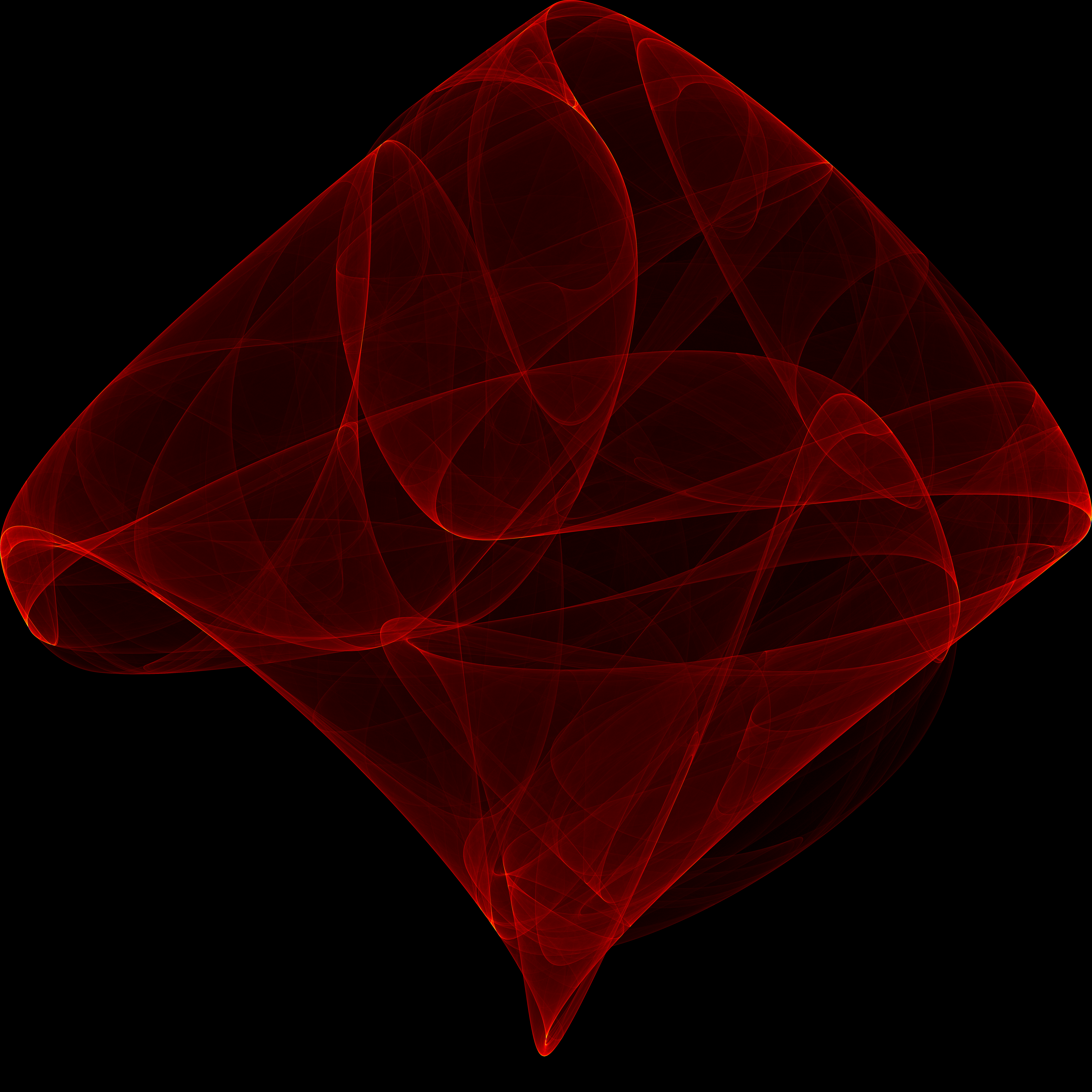
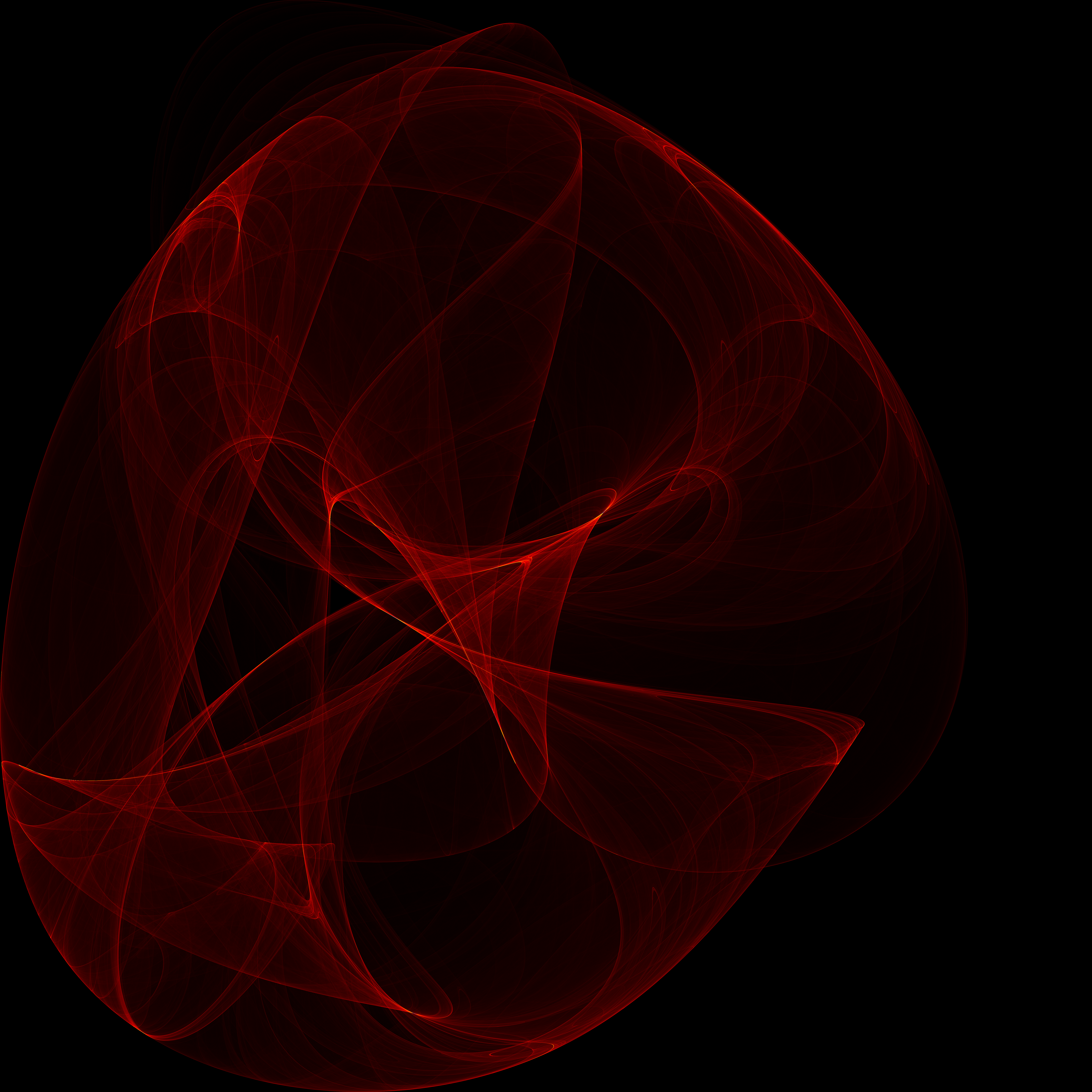
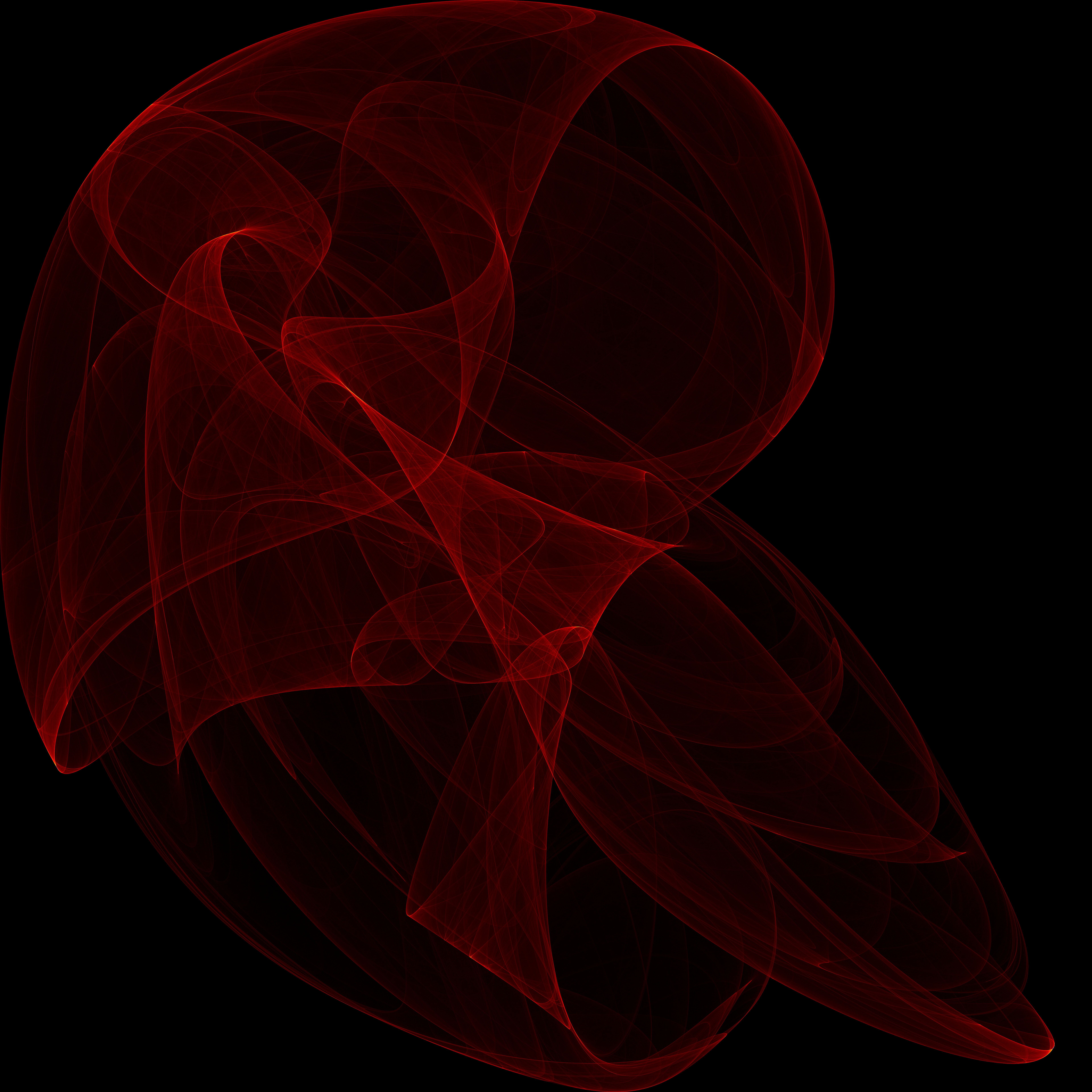
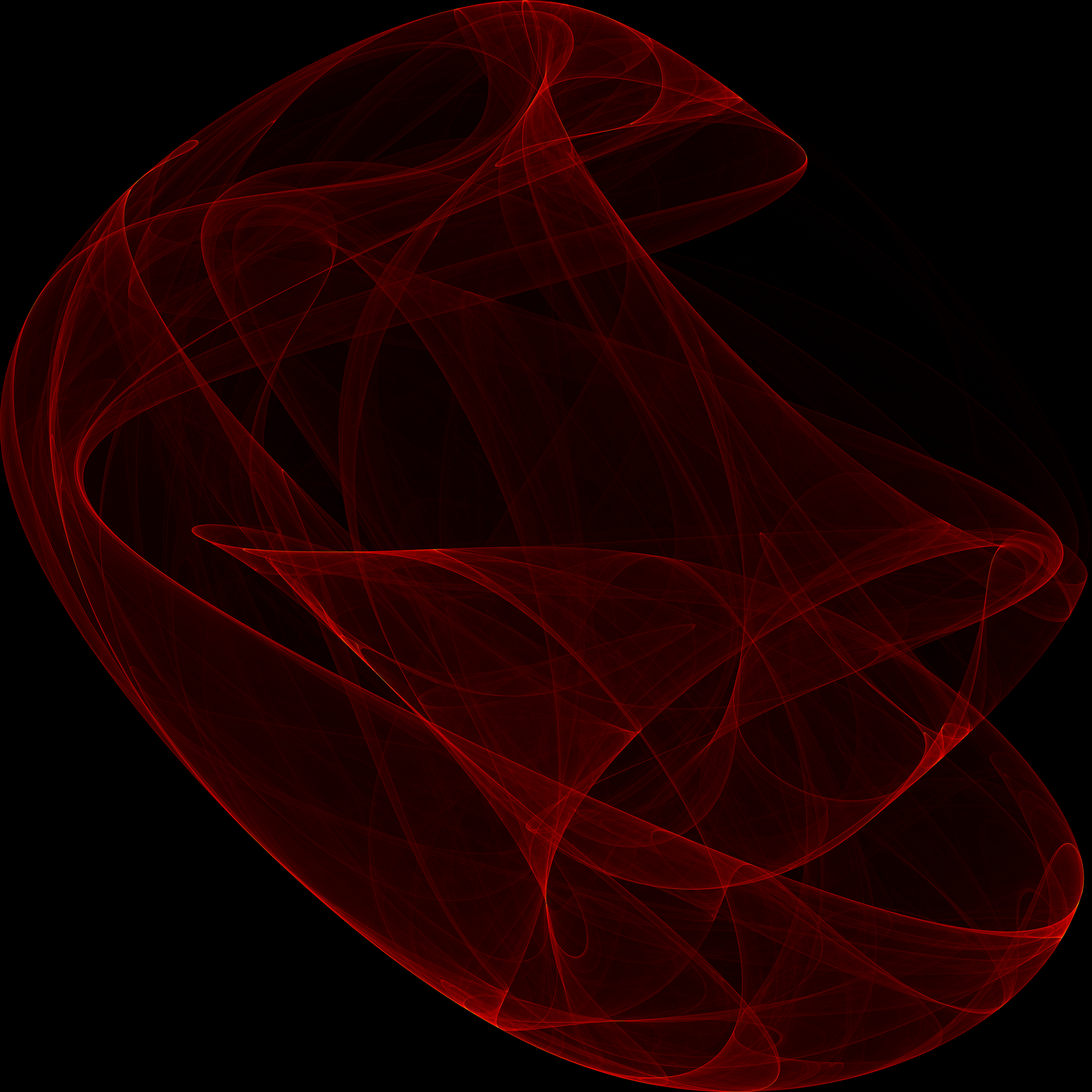
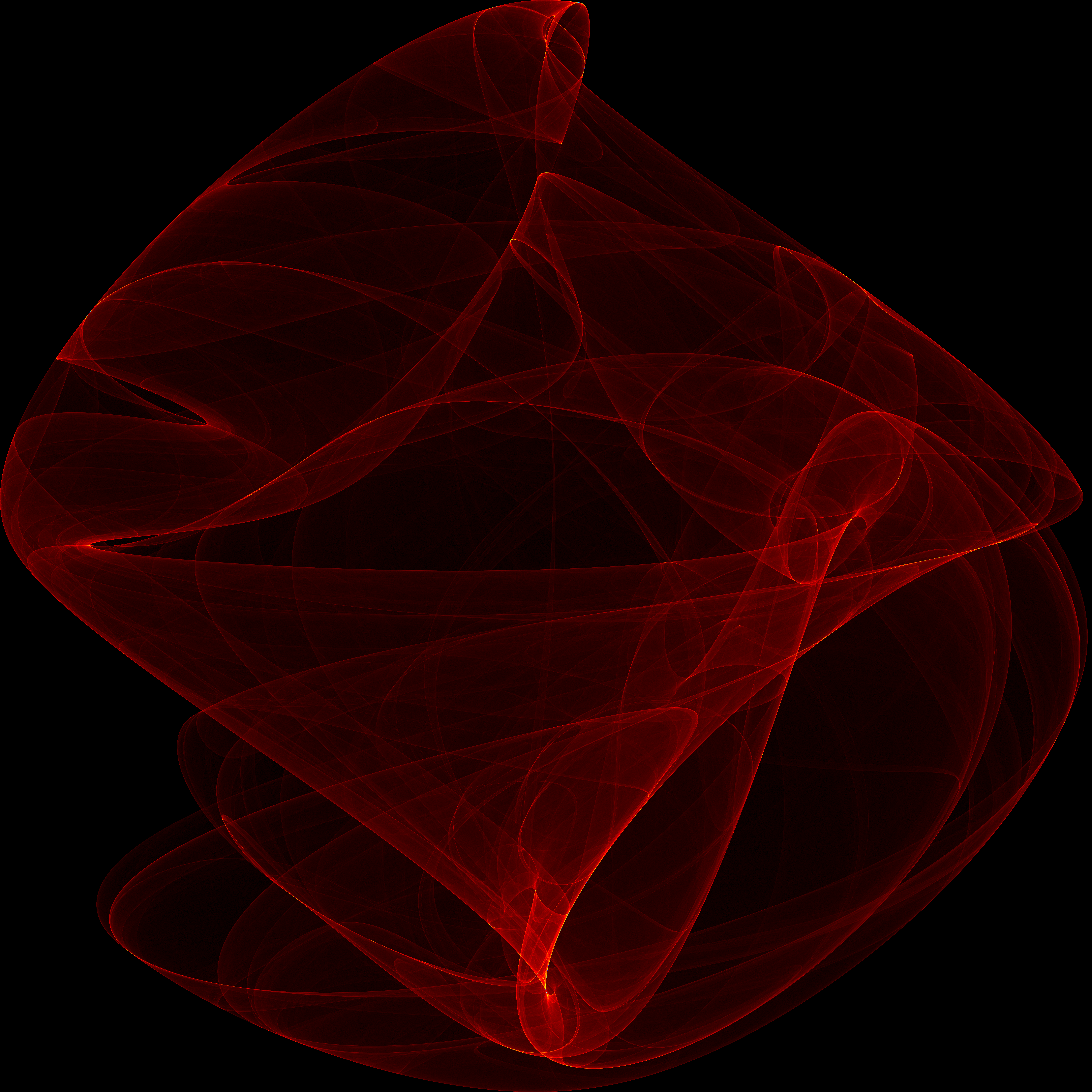
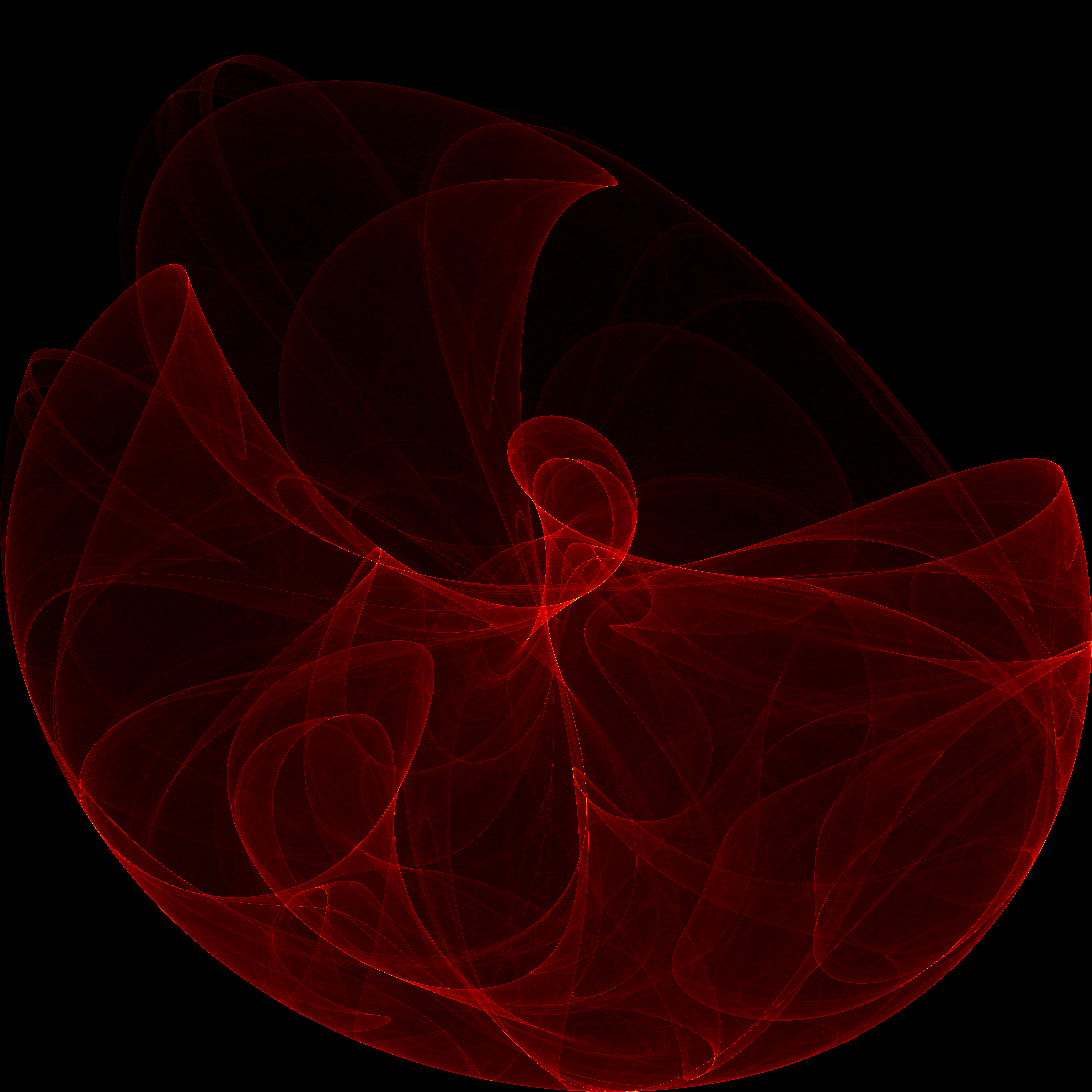
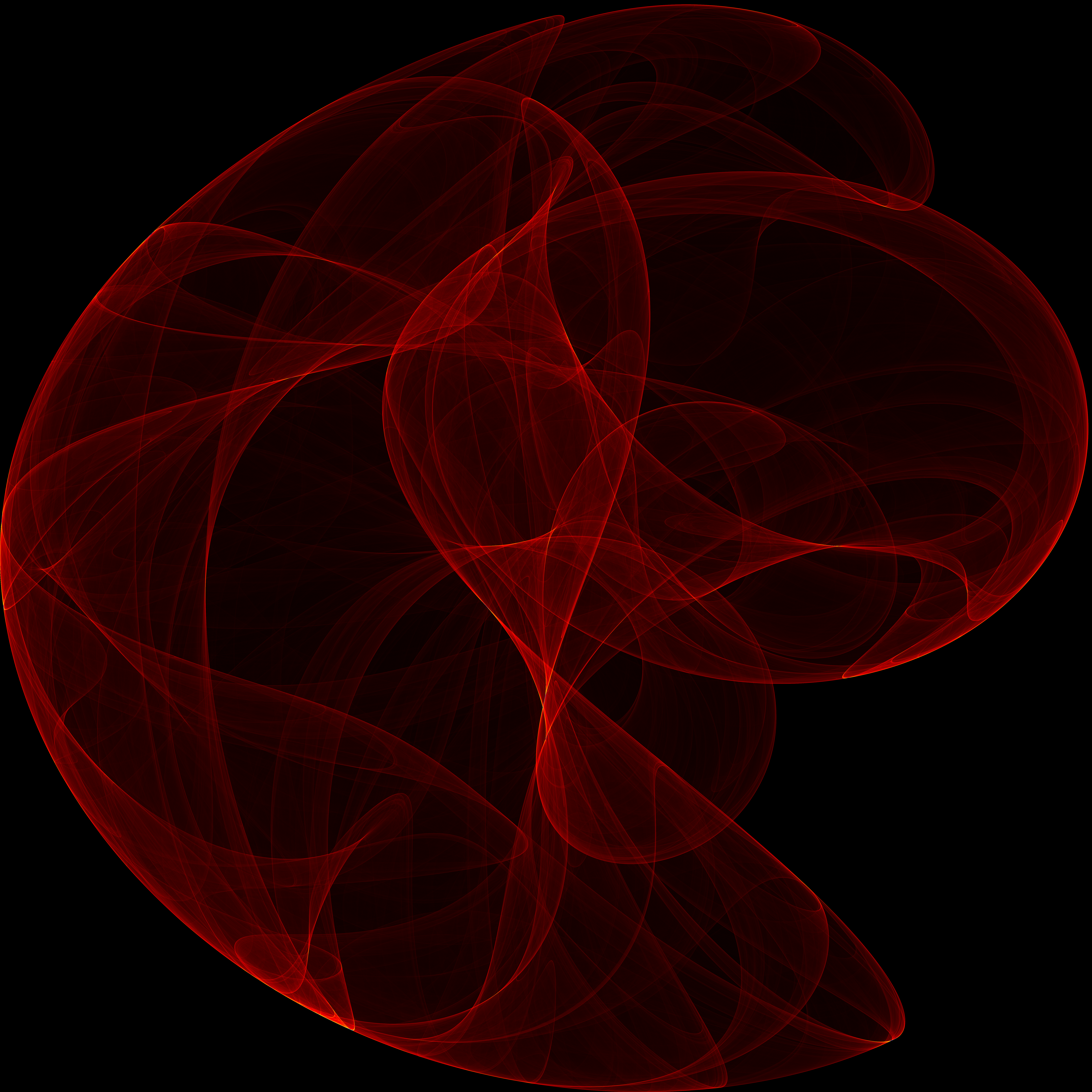
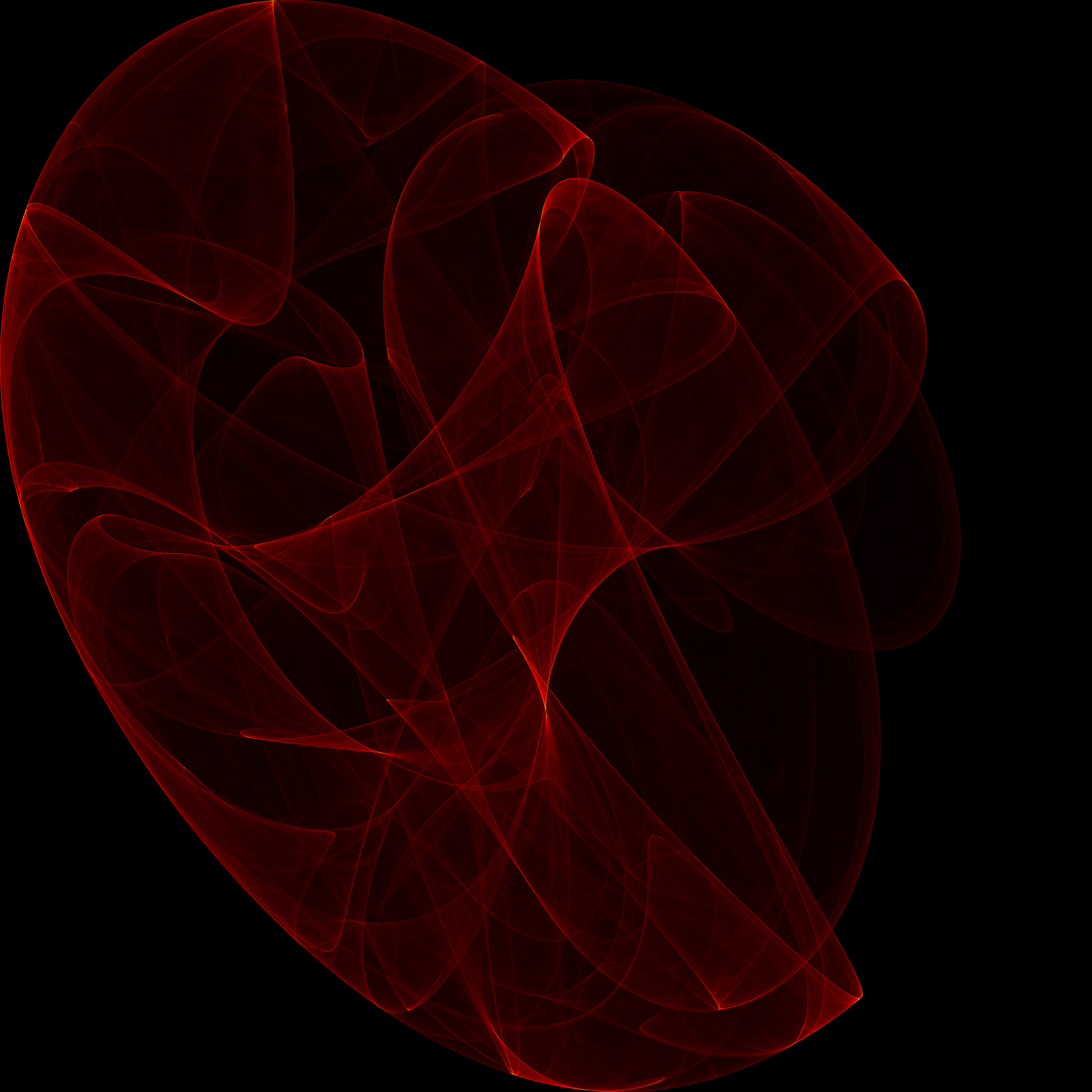
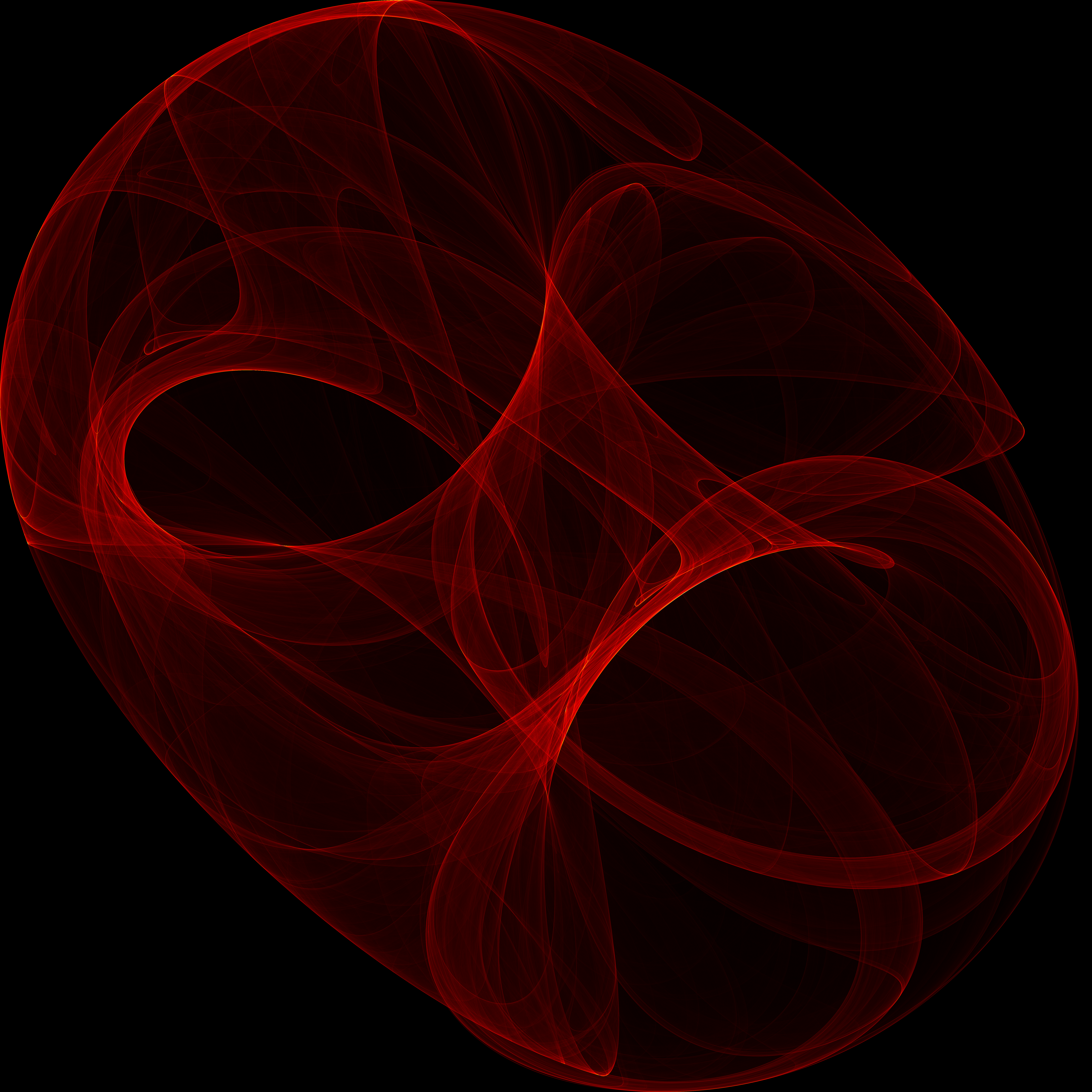
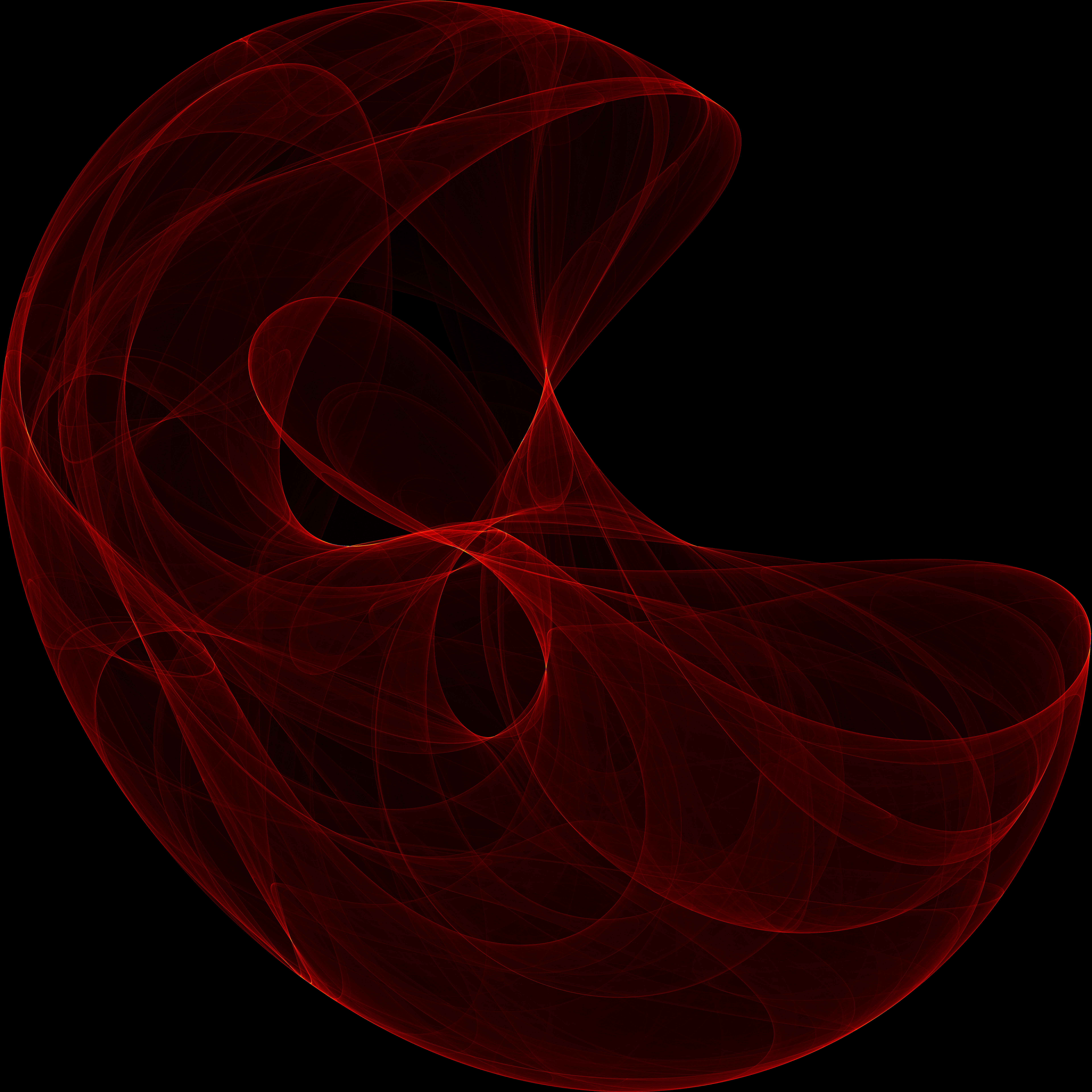
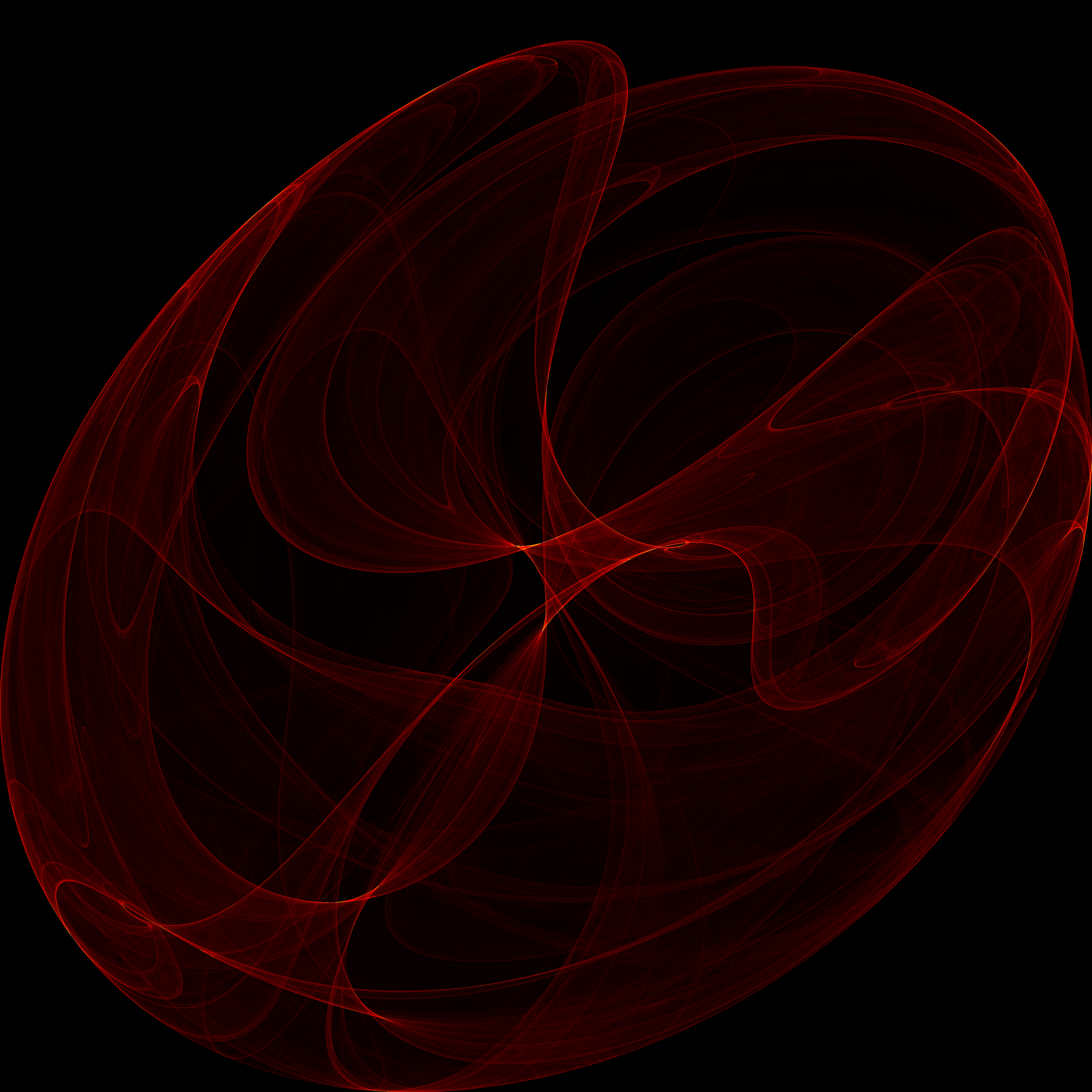
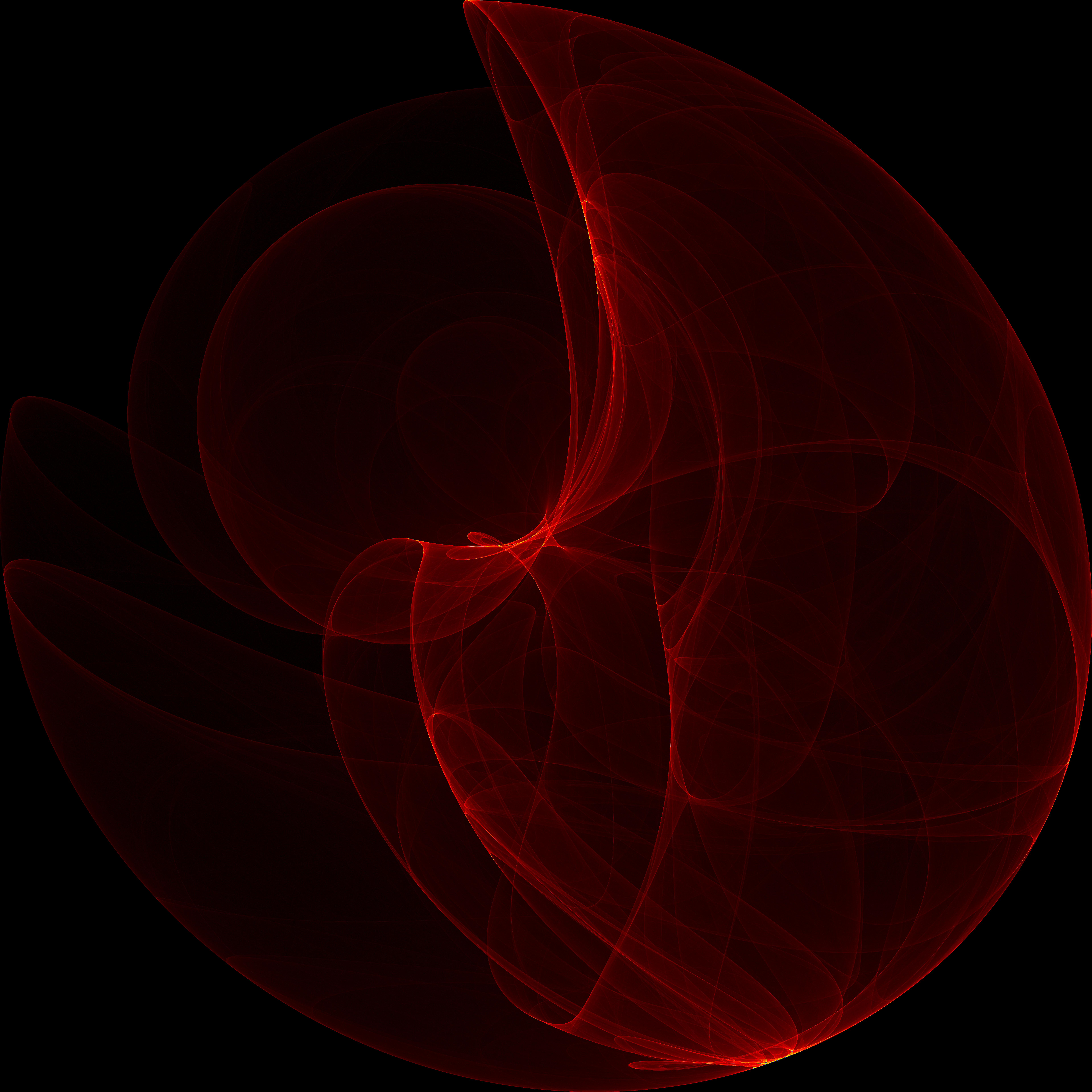
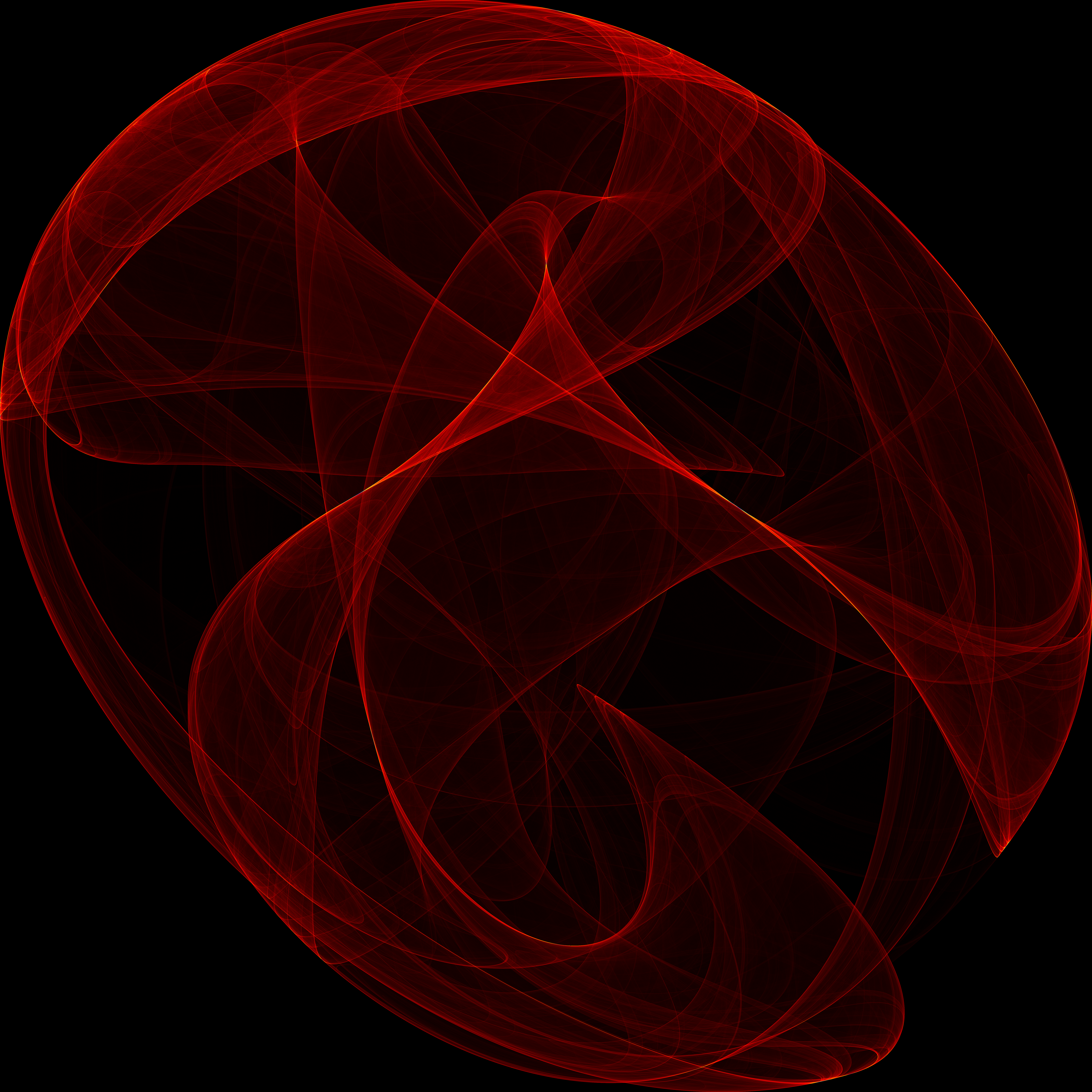
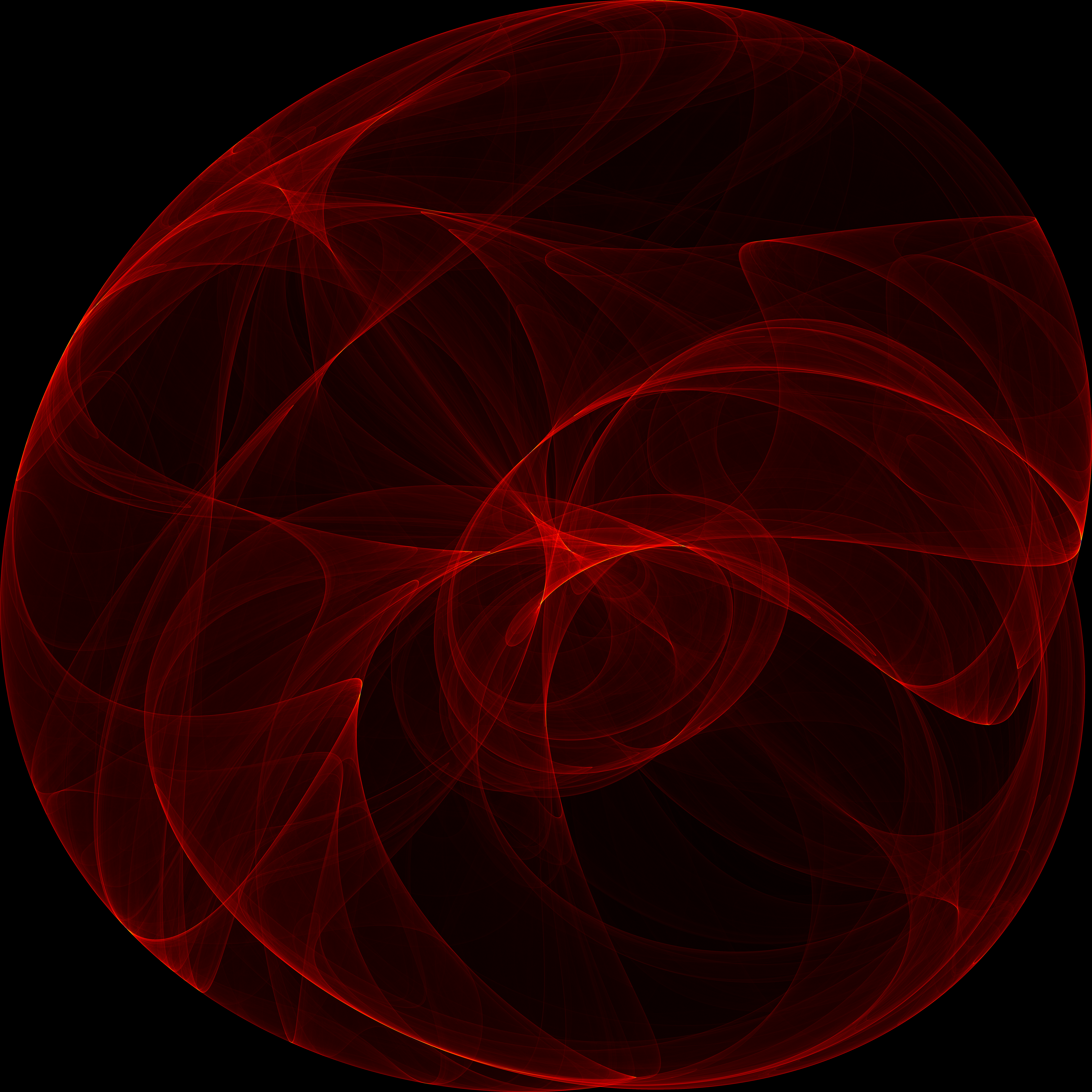
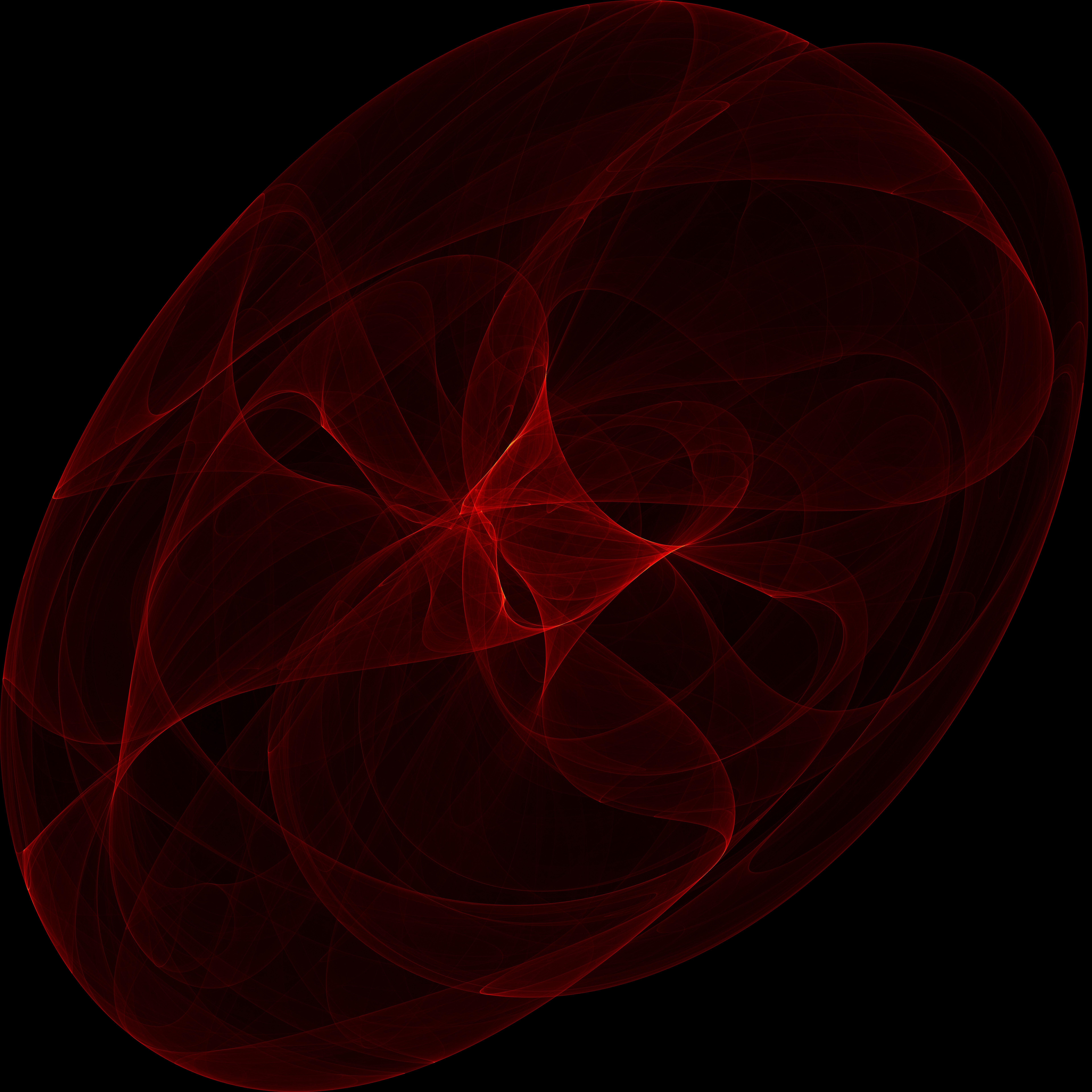
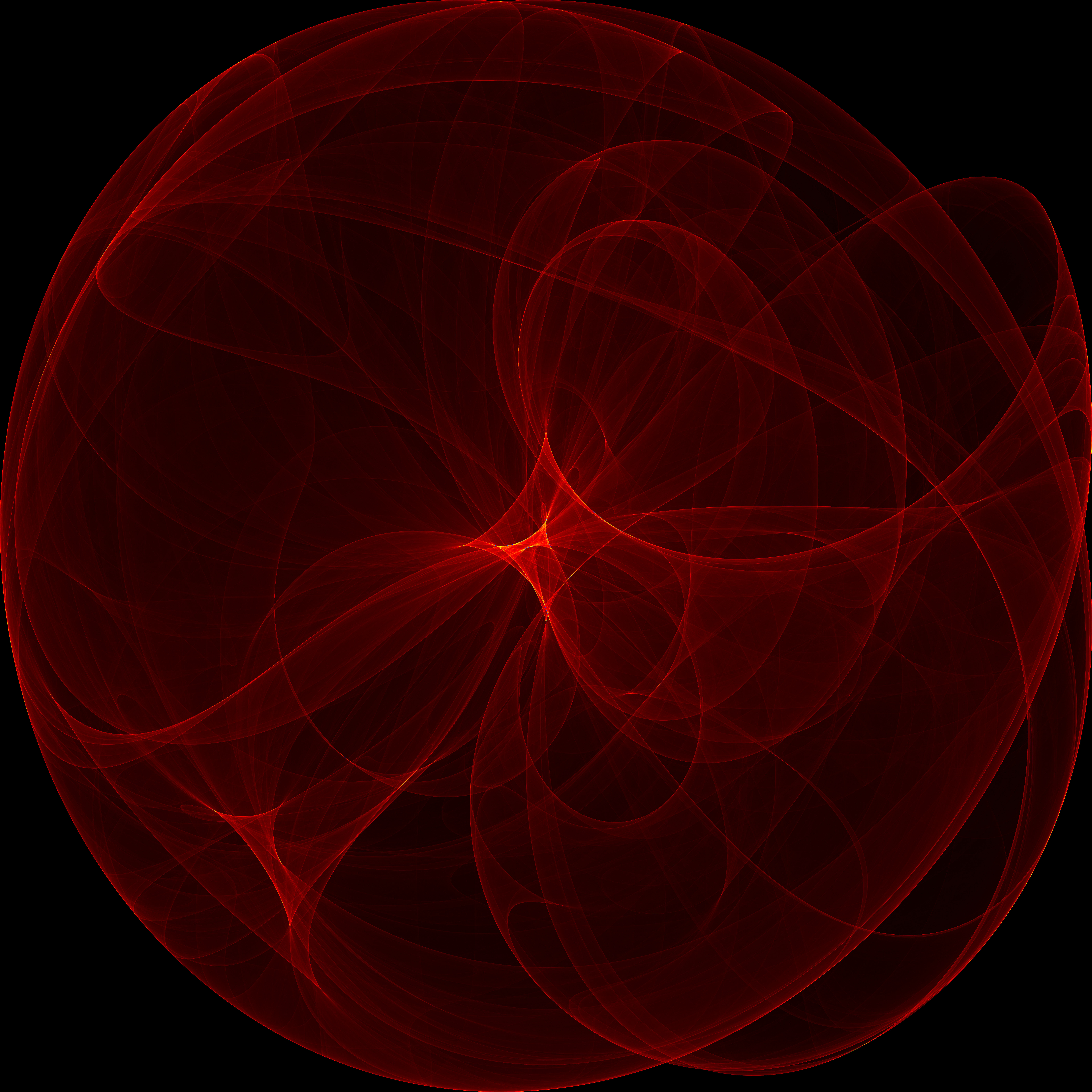
3. Gallery
Here are a few examples. Most of these were discovered via an automated search program using the technique briefly outlined in the next section. When you draw one of these images with a random set of parameters, the odds are that you are the first human being ever to see that precise image – with four, 32-bit parameters the odds of someone else picking the same parameters is 1 in 2^128.

4. Image Generation: Practical Matters
The first practical matter we must work out is the rectangular region over which we wish to visualize our PDF. We can begin by noticing that the Peter de Jong map is bounded by a circle of radius 2 centered at the origin. Therefore we may always start with the rectangular region \([-2, 2]\times[-2, 2]\).
The next practical consideration is how to color each point in the image. The traditional approach for visualizing a 2D histogram is to allow the probability at each point to be represented by color selected from one of the many color scales used for scientific visualization. The color scale I have used for the images here is a simple color gradient with 6 control points: black, red, yellow, blue, cyan, and white.
Representing the probability with color is a fine choice, but the PDF of the Peter de Jong map presents us with a difficulty. The range of values is quite skewed toward the 0 end of the probability range with very few pixels near the 1 end of the range. The standard answer for this problem is to use a logarithmic scale, but I have elected to preform a root transformation on the base results before applying the color scale.
The same color schemes and power transforms may not work for all of the histograms we wish to visualize, and sometimes it is useful to interactively experiment with various choices – without recomputing all the map values. To this end, I also dump out a grayscale image with actual counts for each pixel so we can load the image up in a tool like ImageJ.
Related to the color scheme are two new questions: 1) How many points do we compute, and 2) How large should the image be (how many pixels). At first, these two questions may not seem to relate to the color scheme; however, they are both critical for a good color image. The answer I have been using for the first question is to stop when the intensity (hit count) of any pixel in the image reaches a cut-toff value. I have had good luck with the value 16383. The intensity, or pixel hit count, is very much influenced by the area (in terms of real coordinates) of each pixel. Fewer pixels, mean we compute many fewer iterates. Smaller pixels, mean computing many more iterations and generating an image with a more complex, rich structure. I have been using an image size of 7680x7680 – 7680 is the horizontal resolution of 8K UHD displays.
Lastly, we must find parameters (\(a\), \(b\), \(c\), and \(d\)) which generate interesting images. The approach I have taken is to search for parameters by selecting random values for the parameters, plotting 10,000 points, and printing out the parameter sets which seem to hit the highest number of unique points.
5. Code
The source code used to generate the images on this page is distributed with the mraster library as one of the examples.
6. References
Check out the fractals section of my reading list.
Also check out Paul Bourke's web page