mrkiss_solvers_wt Module Reference

Solvers. More...

Data Types
interface	deq_iface
	Type for ODE dydt functions. More...
interface	sdf_iface
	Type SDF function on a solution point. More...
interface	stepp_iface
	Type step processing subroutine. More...

Functions/Subroutines
One Step Solvers
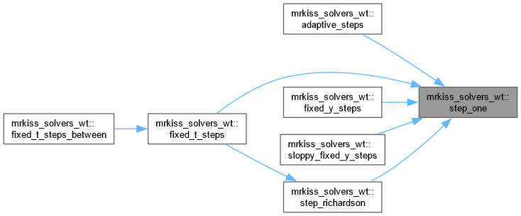
subroutine, public	step_all (status, y_deltas, dy, deq, t, y, param, a, b, c, t_delta)
	Compute one step of a embedded Runge-Kutta method expressed as a Butcher Tableau.
subroutine, public	step_one (status, y_delta, dy, deq, t, y, param, a, b, c, t_delta)
	Compute one step of a Runge-Kutta method expressed as a Butcher Tableau.
subroutine, public	step_richardson (status, y_delta, dy, deq, t, y, param, a, b, c, p, t_delta)
	Compute one Richardson Extrapolation Step.
One Step Test Solvers
subroutine, public	step_rk4 (status, y_delta, dy, deq, t, y, param, t_delta)
	Compute one step of RK4 – the classical 4th order Runge-Kutta method (mrkiss_erk_kutta_4).
subroutine, public	step_rkf45 (status, y_deltas, dy, deq, t, y, param, t_delta)
	Compute one step of RKF45 (mrkiss_eerk_fehlberg_4_5).
subroutine, public	step_dp54 (status, y_deltas, dy, deq, t, y, param, t_delta)
	Compute one step of DP45 (mrkiss_eerk_dormand_prince_5_4)
Multistep Solvers
subroutine, public	fixed_t_steps (status, istats, solution, deq, t, y, param, a, b, c, p_o, max_pts_o, t_delta_o, t_end_o, t_max_o)
	Take multiple fixed time steps with a simple Runge-Kutta method.
subroutine, public	fixed_y_steps (status, istats, solution, deq, t, y, param, a, b, c, y_delta_len_targ, t_delta_max, t_delta_min_o, y_delta_len_tol_o, max_bisect_o, no_bisect_error_o, y_delta_len_idxs_o, max_pts_o, y_sol_len_max_o, t_max_o)
	Take multiple adaptive steps with constant \(\mathbf{\Delta{y}}\) length using a simple Runge-Kutta method.
subroutine, public	sloppy_fixed_y_steps (status, istats, solution, deq, t, y, param, a, b, c, y_delta_len_targ, t_delta_ini, t_max_o, t_delta_min_o, t_delta_max_o, y_delta_len_idxs_o, adj_short_o, max_pts_o, y_sol_len_max_o)
	Take multiple adaptive steps adjusting for the length of \(\mathbf{\Delta{y}}\) using a simple Runge-Kutta method.
subroutine, public	adaptive_steps (status, istats, solution, deq, t, y, param, a, b, c, p, t_max_o, t_end_o, t_delta_ini_o, t_delta_min_o, t_delta_max_o, t_delta_fac_min_o, t_delta_fac_max_o, t_delta_fac_fdg_o, error_tol_abs_o, error_tol_rel_o, max_pts_o, max_bisect_o, no_bisect_error_o, sdf_o, sdf_tol_o, stepp_o)
	Take multiple adaptive steps with an embedded Runge-Kutta method using relatively traditional step size controls.
Multistep Meta Solvers
subroutine, public	fixed_t_steps_between (status, istats, solution, deq, y, param, a, b, c, steps_per_pnt, p_o)
	Take a solution with \(t\) values pre-populated, and take steps_per_pnt Runge-Kutta steps between each \(t\) value.
subroutine, public	interpolate_solution (status, istats, solution, src_solution, deq, param, num_src_pts_o, linear_interp_o)
	Create an interpolated solution from a source solution.

Detailed Description

Solvers.

Function/Subroutine Documentation

step_all()

subroutine, public mrkiss_solvers_wt::step_all	(	integer, intent(out)	status,
		real(kind=rk), dimension(:,:), intent(out)	y_deltas,
		real(kind=rk), dimension(:), intent(out)	dy,
		procedure(deq_iface)	deq,
		real(kind=rk), intent(in)	t,
		real(kind=rk), dimension(:), intent(in)	y,
		real(kind=rk), dimension(:), intent(in)	param,
		real(kind=rk), dimension(:,:), intent(in)	a,
		real(kind=rk), dimension(:,:), intent(in)	b,
		real(kind=rk), dimension(:), intent(in)	c,
		real(kind=rk), intent(in)	t_delta )

Compute one step of a embedded Runge-Kutta method expressed as a Butcher Tableau.

Parameters

status	Exit status Value Description -inf-0 Everything worked 0-255 Evaluation of deq failed 1232-1247 Unknown error in this routine
y_deltas	Returned \(\mathbf{\Delta{y}}\) values(s) for the method
dy	Returned \(\mathbf{y}'\) value at \(t\)
deq	The equation subroutine returning values for \(\mathbf{y}'\) – i.e. \(\mathbf{f}(t, \mathbf{y})\)
t	Initial condition for \(t\) – i.e. \(t_0\).
y	Initial condition for \(\mathbf{y}\) – i.e. \(\mathbf{y_0}\).
param	Data payload passed to deq
a	The butcher tableau \(\mathbf{a}\) matrix
b	The butcher tableau \(\mathbf{b}\) vector
c	The butcher tableau \(\mathbf{c}\) vector
t_delta	The \(\Delta{t}\) value for this step.

Definition at line 152 of file mrkiss_solvers_wt.f90.

Here is the caller graph for this function:

step_one()

subroutine, public mrkiss_solvers_wt::step_one	(	integer, intent(out)	status,
		real(kind=rk), dimension(:), intent(out)	y_delta,
		real(kind=rk), dimension(:), intent(out)	dy,
		procedure(deq_iface)	deq,
		real(kind=rk), intent(in)	t,
		real(kind=rk), dimension(:), intent(in)	y,
		real(kind=rk), dimension(:), intent(in)	param,
		real(kind=rk), dimension(:,:), intent(in)	a,
		real(kind=rk), dimension(:,:), intent(in)	b,
		real(kind=rk), dimension(:), intent(in)	c,
		real(kind=rk), intent(in)	t_delta )

Compute one step of a Runge-Kutta method expressed as a Butcher Tableau.

Parameters

status	Exit status Value Description -inf-0 Everything worked 0-255 Evaluation of deq failed 1232-1247 Unknown error in this routine
y_delta	Returned \(\mathbf{\Delta{y}}\) value for the method
dy	Returned \(\mathbf{y}'\) value at \(t\)
deq	The equation subroutine returning values for \(\mathbf{y}'\) – i.e. \(\mathbf{f}(t, \mathbf{y})\)
t	Initial condition for \(t\) – i.e. \(t_0\).
y	Initial condition for \(\mathbf{y}\) – i.e. \(\mathbf{y_0}\).
param	Data payload passed to deq
a	The butcher tableau \(\mathbf{a}\) matrix
b	The butcher tableau \(\mathbf{b}\) vector
c	The butcher tableau \(\mathbf{c}\) vector
t_delta	The \(\Delta{t}\) value for this step.

Definition at line 207 of file mrkiss_solvers_wt.f90.

Here is the caller graph for this function:

step_richardson()

subroutine, public mrkiss_solvers_wt::step_richardson	(	integer, intent(out)	status,
		real(kind=rk), dimension(:), intent(out)	y_delta,
		real(kind=rk), dimension(:), intent(out)	dy,
		procedure(deq_iface)	deq,
		real(kind=rk), intent(in)	t,
		real(kind=rk), dimension(:), intent(in)	y,
		real(kind=rk), dimension(:), intent(in)	param,
		real(kind=rk), dimension(:,:), intent(in)	a,
		real(kind=rk), dimension(:,:), intent(in)	b,
		real(kind=rk), dimension(:), intent(in)	c,
		integer, dimension(:), intent(in)	p,
		real(kind=rk), intent(in)	t_delta )

Compute one Richardson Extrapolation Step.

This routine produces an improved value for \(\mathbf{\Delta{y}}\), whch we denote by \(\mathbf{\Delta{\tilde{y}}}\), by combining two approximations of \(\mathbf{\Delta{y}}\). If the original Runge-Kutta method was \(\mathcal{O}(p)\), then this new approximation is \(\mathcal{O}(p+1)\). The first approximation of \(\mathbf{\Delta{y}}\), which we denote by \(\mathbf{\Delta{y_B}}\), is computed in the standard way with a single Runge-Kutta step of size \(\Delta{t}\). The second approximation of \(\mathbf{\Delta{y}}\), which we denote by \(\mathbf{\Delta{y_S}}\), is computed by taking two Runge-Kutta steps of size \(\frac{\Delta{t}}{2}\). We combine these approximations to compute our improved \(\mathbf{\Delta{y}}\) as follows:

\[ \mathbf{\Delta{\tilde{y}}} = \mathbf{\Delta{y_S}} + \frac{\mathbf{\Delta{y_S}} - \mathbf{\Delta{y_B}}}{2^p - 1} \]

Parameters

status	Exit status Value Description -inf-0 Everything worked 0-255 Evaluation of deq failed 1216-1231 Unknown error in this routine 1248-1263 Error from mrkiss_solvers_wt::step_one()
y_delta	Returned \(\mathbf{\Delta{y}}\) for the method
dy	Returned \(\mathbf{y}'\) value at \(t\)
deq	The equation subroutine returning values for \(\mathbf{y}'\) – i.e. \(\mathbf{f}(t, \mathbf{y})\)
t	Initial condition for \(t\) – i.e. \(t_0\).
y	Initial condition for \(\mathbf{y}\) – i.e. \(\mathbf{y_0}\).
param	Data payload passed to deq
a	The butcher tableau \(\mathbf{a}\) matrix
b	The butcher tableau \(\mathbf{{b}}\) vector
c	The butcher tableau \(\mathbf{c}\) vector
p	The order(s) of the Runge-Kutta methods in the butcher tableau
t_delta	The \(\Delta{t}\) value for this step.

Definition at line 274 of file mrkiss_solvers_wt.f90.

Here is the call graph for this function:

Here is the caller graph for this function:

step_rk4()

subroutine, public mrkiss_solvers_wt::step_rk4	(	integer, intent(out)	status,
		real(kind=rk), dimension(:), intent(out)	y_delta,
		real(kind=rk), dimension(:), intent(out)	dy,
		procedure(deq_iface)	deq,
		real(kind=rk), intent(in)	t,
		real(kind=rk), dimension(:), intent(in)	y,
		real(kind=rk), dimension(:), intent(in)	param,
		real(kind=rk), intent(in)	t_delta )

Compute one step of RK4 – the classical 4th order Runge-Kutta method (mrkiss_erk_kutta_4).

Parameters

status	Exit status Value Description -inf-0 Everything worked 0-255 Evaluation of deq failed 1200-1215 Unknown error in this routine
y_delta	Returned \(\mathbf{\Delta{y}}\) for the method
dy	Returned \(\mathbf{y}'\) value at \(t\)
deq	The equation subroutine returning values for \(\mathbf{y}'\) – i.e. \(\mathbf{f}(t, \mathbf{y})\)
t	Initial condition for \(t\) – i.e. \(t_0\).
y	Initial condition for \(\mathbf{y}\) – i.e. \(\mathbf{y_0}\).
param	Data payload passed to deq
t_delta	The \(\Delta{t}\) value for this step.

Definition at line 325 of file mrkiss_solvers_wt.f90.

step_rkf45()

subroutine, public mrkiss_solvers_wt::step_rkf45	(	integer, intent(out)	status,
		real(kind=rk), dimension(:,:), intent(out)	y_deltas,
		real(kind=rk), dimension(:), intent(out)	dy,
		procedure(deq_iface)	deq,
		real(kind=rk), intent(in)	t,
		real(kind=rk), dimension(:), intent(in)	y,
		real(kind=rk), dimension(:), intent(in)	param,
		real(kind=rk), intent(in)	t_delta )

Compute one step of RKF45 (mrkiss_eerk_fehlberg_4_5).

Parameters

status	Exit status Value Description -inf-0 Everything worked 0-255 Evaluation of deq failed 1184-1199 Unknown error in this routine
y_deltas	Returned \(\mathbf{\Delta{y}}\) values
dy	Returned \(\mathbf{y}'\) value at \(t\)
deq	The equation subroutine returning values for \(\mathbf{y}'\) – i.e. \(\mathbf{f}(t, \mathbf{y})\)
t	Initial condition for \(t\) – i.e. \(t_0\).
y	Initial condition for \(\mathbf{y}\) – i.e. \(\mathbf{y_0}\).
param	Data payload passed to deq
t_delta	The \(\Delta{t}\) value for this step.

Definition at line 366 of file mrkiss_solvers_wt.f90.

step_dp54()

subroutine, public mrkiss_solvers_wt::step_dp54	(	integer, intent(out)	status,
		real(kind=rk), dimension(:,:), intent(out)	y_deltas,
		real(kind=rk), dimension(:), intent(out)	dy,
		procedure(deq_iface)	deq,
		real(kind=rk), intent(in)	t,
		real(kind=rk), dimension(:), intent(in)	y,
		real(kind=rk), dimension(:), intent(in)	param,
		real(kind=rk), intent(in)	t_delta )

Compute one step of DP45 (mrkiss_eerk_dormand_prince_5_4)

Parameters

status	Exit status Value Description -inf-0 Everything worked 0-255 Evaluation of deq failed 1263-1279 Unknown error in this routine
y_deltas	Returned \(\mathbf{\Delta{y}}\) values
dy	Returned \(\mathbf{y}'\) value at \(t\)
deq	The equation subroutine returning values for \(\mathbf{y}'\) – i.e. \(\mathbf{f}(t, \mathbf{y})\)
t	Initial condition for \(t\) – i.e. \(t_0\).
y	Initial condition for \(\mathbf{y}\) – i.e. \(\mathbf{y_0}\).
param	Data payload passed to deq
t_delta	The \(\Delta{t}\) value for this step.

Definition at line 414 of file mrkiss_solvers_wt.f90.

fixed_t_steps()

subroutine, public mrkiss_solvers_wt::fixed_t_steps	(	integer, intent(out)	status,
		integer, dimension(istats_size), intent(out)	istats,
		real(kind=rk), dimension(:,:), intent(out)	solution,
		procedure(deq_iface)	deq,
		real(kind=rk), intent(in)	t,
		real(kind=rk), dimension(:), intent(in)	y,
		real(kind=rk), dimension(:), intent(in)	param,
		real(kind=rk), dimension(:,:), intent(in)	a,
		real(kind=rk), dimension(:,:), intent(in)	b,
		real(kind=rk), dimension(:), intent(in)	c,
		integer, dimension(:), intent(in), optional	p_o,
		integer, intent(in), optional	max_pts_o,
		real(kind=rk), intent(in), optional	t_delta_o,
		real(kind=rk), intent(in), optional	t_end_o,
		real(kind=rk), intent(in), optional	t_max_o )

Take multiple fixed time steps with a simple Runge-Kutta method.

Parameters

status	Exit status Value Description -inf-0 Everything worked 0-255 Evaluation of deq failed 1120-1151 Unnecessary error in this routine 1216-1231 Error from mrkiss_solvers_wt::step_richardson() 1248-1263 Error from mrkiss_solvers_wt::step_one()
istats	Integer statistics for run See: mrkiss_config::istats_strs for a description of elements. Elements this routine updates mrkiss_config::isi_num_pts mrkiss_config::isi_one_reg
solution	Array for solution. Each COLUMN is a solution: First element is the \(t\) variable size(y, 1) elements starting with 2 have \(\mathbf{y}\) values The next size(y, 1) elements have \(\mathbf{y}'\) values
deq	The equation subroutine returning values for \(\mathbf{y}'\) – i.e. \(\mathbf{f}(t, \mathbf{y})\)
t	Initial condition for \(t\) – i.e. \(t_0\).
y	Initial condition for \(\mathbf{y}\) – i.e. \(\mathbf{y_0}\).
param	Data payload passed to deq
a	The butcher tableau \(\mathbf{a}\) matrix
b	The butcher tableau \(\mathbf{{b}}\) vector
c	The butcher tableau \(\mathbf{c}\) vector
p_o	The order for the Runge-Kutta method in the butcher tableau to enable Richardson extrapolation
max_pts_o	Maximum number of points to put in solution. If max_pts_o>1 & size(solution, 2)==1, then max_pts_o-1 steps are taken and only the last solution is stored in solution.
t_delta_o	Step size to use. Default when t_end_o provided: (t_end - t) / (size(solution, 2) - 1) Default othewise: mrkiss_config::t_delta_ai
t_end_o	End point for last step. Silently ignored if t_delta_o is provided.
t_max_o	Maximum value for \(t\)

Definition at line 488 of file mrkiss_solvers_wt.f90.

Here is the call graph for this function:

Here is the caller graph for this function:

fixed_y_steps()

subroutine, public mrkiss_solvers_wt::fixed_y_steps	(	integer, intent(out)	status,
		integer, dimension(istats_size), intent(out)	istats,
		real(kind=rk), dimension(:,:), intent(out)	solution,
		procedure(deq_iface)	deq,
		real(kind=rk), intent(in)	t,
		real(kind=rk), dimension(:), intent(in)	y,
		real(kind=rk), dimension(:), intent(in)	param,
		real(kind=rk), dimension(:,:), intent(in)	a,
		real(kind=rk), dimension(:,:), intent(in)	b,
		real(kind=rk), dimension(:), intent(in)	c,
		real(kind=rk), intent(in)	y_delta_len_targ,
		real(kind=rk), intent(in)	t_delta_max,
		real(kind=rk), intent(in), optional	t_delta_min_o,
		real(kind=rk), intent(in), optional	y_delta_len_tol_o,
		integer, intent(in), optional	max_bisect_o,
		logical, intent(in), optional	no_bisect_error_o,
		integer, dimension(:), intent(in), optional	y_delta_len_idxs_o,
		integer, intent(in), optional	max_pts_o,
		real(kind=rk), intent(in), optional	y_sol_len_max_o,
		real(kind=rk), intent(in), optional	t_max_o )

Take multiple adaptive steps with constant \(\mathbf{\Delta{y}}\) length using a simple Runge-Kutta method.

This method attempts to precisely control the length of \(\mathbf{\Delta{y}}\) which we denote by \(\vert\vert\mathbf{\Delta{y}}\vert\vert_L\). This is done by finding a value for \(\Delta{t}\) for which \(\vert\vert\mathbf{\Delta{y}}\vert\vert_L\) is equal to y_delta_len_targ with an accuracy of y_delta_len_tol_o.

This value for \(\Delta{t}\) is found via bisection. For each solution point we first compute two Runge-Kutta steps with \(\Delta{t}\) set to t_delta_min_o and t_delta_max. We hope that the lengths of the two \(\mathbf{\Delta{y}}\) values thus obtained will bracket y_delta_len_targ. If they don't then we can't isolate an appropriate value for \(\Delta{t}\). In this case we ignore the issue and continue to the next step if no_bisect_error_o is .TRUE., otherwise we error out with a status code of 1024. If the lengths of our \(\mathbf{\Delta{y}}\) values bracket the target, then we use bisection to localize a value for \(\Delta{t}\).

The length, which we have denoted by \(\vert\vert\mathbf{\Delta{y}}\vert\vert_L\), is defined to be the Euclidean distance of the vector defined by the elements of \(\mathbf{\Delta{y}}\) that are indexed by y_delta_len_idxs_o.

Note there is no mathematical guarantee that a Runge-Kutta step of size t_delta_min_o and t_delta_max will produce solutions that bracket y_delta_len_targ. That said, for well behaved functions a t_delta_min_o and t_delta_max may always be found that work. Usually finding good values are t_delta_min_o and t_delta_max isn't difficult. For challenging cases, a good approach is to use fixed_t_steps() over the interval in question, and then examine the values of \(\vert\vert\mathbf{\Delta{y}}\vert\vert_L\) in the solution via analyze_solution().

My primary use case for this function is to create uniform sphere sweeps for constructive solid geometry applications.

Parameters

status	Exit status Value Description 0 Everything worked 0-255 Evaluation of deq failed (see: deq_iface) 1024 bisection containment anomaly 1025 no_bisect_error_o==0 not present and max_bisect_o violated 1026-1055 Unknown error in this routine 1248-1263 Error from mrkiss_solvers_wt::step_one()
istats	Integer statistics for run See: mrkiss_config::istats_strs for a description of elements. Elements this routine updates mrkiss_config::isi_num_pts mrkiss_config::isi_one_reg mrkiss_config::isi_one_y_len mrkiss_config::isi_bic_max mrkiss_config::isi_bic_bnd
solution	Array for solution. Each COLUMN is a solution: First element is the \(t\) variable size(y, 1) elements starting with 2 have \(\mathbf{y}\) values The next size(y, 1) elements have dy values if
deq	The equation subroutine returning values for \(\mathbf{y}'\) – i.e. \(\mathbf{f}(t, \mathbf{y})\)
t	Initial condition for \(t\) – i.e. \(t_0\).
y	Initial condition for \(\mathbf{y}\) – i.e. \(\mathbf{y_0}\).
param	Data payload passed to deq
a	The butcher tableau \(\mathbf{a}\) matrix
b	The butcher tableau \(\mathbf{{b}}\) vector
c	The butcher tableau \(\mathbf{c}\) vector
y_delta_len_targ	Target length for \(\mathbf{\Delta{y}}\) – i.e. \(\vert\vert\mathbf{\Delta{y}}\vert\vert_L\)
t_delta_max	Maximum \(\Delta{t}\)
t_delta_min_o	Minimum \(\Delta{t}\)
y_delta_len_tol_o	How close we have to get to y_delta_len_targ. Default is y_delta_len_targ/100
y_delta_len_idxs_o	Components of \(\mathbf{\Delta{y}}\) to use for length computation
max_pts_o	Maximum number of points to put in solution.
max_bisect_o	Maximum number of bisection iterations per each step. Default: mrkiss_config::max_bisect_ai
no_bisect_error_o	If .TRUE., then do not exit on bisection errors
y_sol_len_max_o	Maximum length of the solution curve
t_max_o	Maximum value for \(t\)

Definition at line 631 of file mrkiss_solvers_wt.f90.

Here is the call graph for this function:

sloppy_fixed_y_steps()

subroutine, public mrkiss_solvers_wt::sloppy_fixed_y_steps	(	integer, intent(out)	status,
		integer, dimension(istats_size), intent(out)	istats,
		real(kind=rk), dimension(:,:), intent(out)	solution,
		procedure(deq_iface)	deq,
		real(kind=rk), intent(in)	t,
		real(kind=rk), dimension(:), intent(in)	y,
		real(kind=rk), dimension(:), intent(in)	param,
		real(kind=rk), dimension(:,:), intent(in)	a,
		real(kind=rk), dimension(:,:), intent(in)	b,
		real(kind=rk), dimension(:), intent(in)	c,
		real(kind=rk), intent(in)	y_delta_len_targ,
		real(kind=rk), intent(in)	t_delta_ini,
		real(kind=rk), intent(in), optional	t_max_o,
		real(kind=rk), intent(in), optional	t_delta_min_o,
		real(kind=rk), intent(in), optional	t_delta_max_o,
		integer, dimension(:), intent(in), optional	y_delta_len_idxs_o,
		integer, intent(in), optional	adj_short_o,
		integer, intent(in), optional	max_pts_o,
		real(kind=rk), intent(in), optional	y_sol_len_max_o )

Take multiple adaptive steps adjusting for the length of \(\mathbf{\Delta{y}}\) using a simple Runge-Kutta method.

This method attempts to control the length of \(\mathbf{\Delta{y}}\) which we denote by \(\vert\vert\mathbf{\Delta{y}}\vert\vert_L\). At each solution step it takes a probing step with \(\Delta{t}\) equal to t_delta_ini and then takes another step with \(\Delta{t}\) equal to: t_delta_ini * y_delta_len_targ / y_delta_len

If which will result in a \(\vert\vert\mathbf{\Delta{y}}\vert\vert_L\) approximately y_delta_len_targ when \(\Delta{t}\) is proportional to \(\vert\vert\mathbf{\Delta{y}}\vert\vert_L\). By default this second step is only taken when \(\vert\vert\mathbf{\Delta{y}}\vert\vert_L\) of the probe step is greater than y_delta_len_targ; however, it will be performed on shorter steps when adj_short_o is present – in this mode it approximates the behavior fixed_y_steps() but is much faster.

Note the assumption that \(\Delta{t}\) is proportional to \(\vert\vert\mathbf{\Delta{y}}\vert\vert_L\). We have no mathematical guarantee for this assumption; however, it is a fair approximation with well behaved functions when t_delta_ini is small enough.

The length, which we have denoted by \(\vert\vert\mathbf{\Delta{y}}\vert\vert_L\), is defined to be the Euclidean distance of the vector defined by the elements of \(\mathbf{\Delta{y}}\) that are indexed by y_delta_len_idxs_o.

My primary use case for this function is to shrink down long steps for smoother curves/tubes in visualizations.

Parameters

status	Exit status Value Description -inf-0 Everything worked 0-255 Evaluation of deq failed 1280-1296 Unknown error in this routine 1248-1263 Error from mrkiss_solvers_wt::step_one()
istats	Integer statistics for run See: mrkiss_config::istats_strs for a description of elements. Elements this routine updates: mrkiss_config::isi_num_pts mrkiss_config::isi_one_reg mrkiss_config::isi_one_y_len
solution	Array for solution. Each COLUMN is a solution: First element is the \(t\) variable size(y, 1) elements starting with 2 have \(\mathbf{y}\) values The next size(y, 1) elements have \(\mathbf{y}'\) values
deq	The equation subroutine returning values for \(\mathbf{y}'\) – i.e. \(\mathbf{f}(t, \mathbf{y})\)
t	Initial condition for \(t\) – i.e. \(t_0\).
y	Initial condition for \(\mathbf{y}\) – i.e. \(\mathbf{y_0}\).
param	Data payload passed to deq
a	The butcher tableau \(\mathbf{a}\) matrix
b	The butcher tableau \(\mathbf{{b}}\) vector
c	The butcher tableau \(\mathbf{c}\) vector
y_delta_len_targ	Target length for \(\mathbf{\Delta{y}}\) – i.e. \(\vert\vert\mathbf{\Delta{y}}\vert\vert_L\)
t_delta_ini	Test step \(\Delta{t}\)
t_delta_max_o	Maximum \(\Delta{t}\)
t_delta_min_o	Minimum \(\Delta{t}\)
y_delta_len_idxs_o	Components of \(\mathbf{\Delta{y}}\) to use for length computation
adj_short_o	Adjust when \(\Delta{t}\) is too short as well as when it's too long.
max_pts_o	Maximum number of points to put in solution.
y_sol_len_max_o	Maximum length of the solution curve
t_max_o	Maximum value for \(t\)

Definition at line 835 of file mrkiss_solvers_wt.f90.

Here is the call graph for this function:

adaptive_steps()

subroutine, public mrkiss_solvers_wt::adaptive_steps	(	integer, intent(out)	status,
		integer, dimension(istats_size), intent(out)	istats,
		real(kind=rk), dimension(:,:), intent(out)	solution,
		procedure(deq_iface)	deq,
		real(kind=rk), intent(in)	t,
		real(kind=rk), dimension(:), intent(in)	y,
		real(kind=rk), dimension(:), intent(in)	param,
		real(kind=rk), dimension(:,:), intent(in)	a,
		real(kind=rk), dimension(:,:), intent(in)	b,
		real(kind=rk), dimension(:), intent(in)	c,
		integer, dimension(:), intent(in)	p,
		real(kind=rk), intent(in), optional	t_max_o,
		real(kind=rk), intent(in), optional	t_end_o,
		real(kind=rk), intent(in), optional	t_delta_ini_o,
		real(kind=rk), intent(in), optional	t_delta_min_o,
		real(kind=rk), intent(in), optional	t_delta_max_o,
		real(kind=rk), intent(in), optional	t_delta_fac_min_o,
		real(kind=rk), intent(in), optional	t_delta_fac_max_o,
		real(kind=rk), intent(in), optional	t_delta_fac_fdg_o,
		real(kind=rk), dimension(:), intent(in), optional	error_tol_abs_o,
		real(kind=rk), dimension(:), intent(in), optional	error_tol_rel_o,
		integer, intent(in), optional	max_pts_o,
		integer, intent(in), optional	max_bisect_o,
		logical, intent(in), optional	no_bisect_error_o,
		procedure(sdf_iface), optional	sdf_o,
		real(kind=rk), intent(in), optional	sdf_tol_o,
		procedure(stepp_iface), optional	stepp_o )

Take multiple adaptive steps with an embedded Runge-Kutta method using relatively traditional step size controls.

Method of controlling step size:

First we compute a combined tolerance vector:

\[ \mathbf{E} = [ A_i + R_i \max(\vert y_i\vert, \vert y_i+\Delta t\vert) ] \]

Now define a set containing the indexes of the non-zero elements of \(\mathbf{E}\):

\[ \mathbf{E_+} = \{i\vert\,E_i\ne0\} \]

When \(\vert E_+\vert=0\), i.e. when \(E_+=\emptyset\):

• We accept the current step
• Expand the next step by a factor of t_delta_fac_max_o

Otherwise, we compute a composite error estimate:

\[ \epsilon = \sqrt{\frac{1}{\vert E_+\vert} \sum_{E_+}\left(\frac{\vert\Delta{y}_i-\Delta{y}_i\vert}{E_i}\right)^2} \]

From this we compute the ideal step size adjustment ratio:

\[ m = \left(\frac{1}{\epsilon}\right)^\frac{1}{1+\min(\p, \check{p})} \]

When \( \vert\Delta{y}_i-\Delta{y}_i\vert < E_i\,\,\,\,\forall i\), we:

• We accept the current step
• Expand the next step by a factor of \(m\)

Otherwise

• We recompute the current step with a \(\Delta{t}\) reduced by \(m\)
• Recompute the error conditions
• Set the next step size based on the error conditions

Notes:

• When \(m<1\), the factor is adjusted by t_delta_fac_fdg_o
• The final value for \(m\) is constrained by t_delta_fac_max_o & t_delta_fac_min_o.
• The final value for \(\Delta{t}\) is always constrained by t_delta_min_o & t_delta_max_o.
• This routine is sensitive to compiler optimizations. For example, ifx requires -fp-model=precise in order to insure consistent results with other compilers – the results without this option are not incorrect, just different.

Parameters

status	Exit status Value Description -inf-0 Everything worked 0-255 Evaluation of deq failed 256-511 Error in stepp_o 512-767 Error in sdf_o 1056 no_bisect_error_o is .FALSE. and max_bisect_o violated. 1057-1119 Unknown error in this routine 1232-1247 Error from mrkiss_solvers_wt::step_all() 1248-1263 Error from mrkiss_solvers_wt::step_one()
istats	Integer statistics for run See: mrkiss_config::istats_strs for a description of elements. Elements this routine updates: mrkiss_config::isi_num_pts mrkiss_config::isi_all_norm mrkiss_config::isi_all_y_err mrkiss_config::isi_one_spp_td mrkiss_config::isi_sdf_step mrkiss_config::isi_bic_max mrkiss_config::isi_bic_bnd
solution	Array for solution. Each COLUMN is a solution: First element is the \(t\) variable size(y, 1) elements starting with 2 have \(\mathbf{y}\) values The next size(y, 1) elements have \(\mathbf{y}'\) values
deq	The equation subroutine returning values for \(\mathbf{y}'\) – i.e. \(\mathbf{f}(t, \mathbf{y})\)
t	Initial condition for \(t\) – i.e. \(t_0\).
y	Initial condition for \(\mathbf{y}\) – i.e. \(\mathbf{y_0}\).
param	Data payload passed to deq
a	The butcher tableau \(\mathbf{a}\) matrix
b	The butcher tableau \(\mathbf{b}\) vector
c	The butcher tableau \(\mathbf{c}\) vector
p	Orders for the methods in the butcher tableau
t_max_o	Stop if \(t\) becomes greater than t_max_o. Different from t_end_o! Default: NONE
t_end_o	Try to stop integration with \(t\) equal to t_end. Default: NONE
t_delta_ini_o	Initial \(\Delta{t}\). Default when t_delta_max provided: (t_delta_max_o+t_delta_min_o)/2 Default otherwise: mrkiss_config::t_delta_ai
t_delta_min_o	Minimum allowed \(\Delta{t}\). Default: mrkiss_config::t_delta_min_ai
t_delta_max_o	Maximum allowed \(\Delta{t}\). Default: NONE
t_delta_fac_min_o	Minimum \(\Delta{t}\) adaption factor for all but the first step. Default: mrkiss_config::t_delta_fac_min_ai
t_delta_fac_max_o	Maximum \(\Delta{t}\) adaption factor. Default: 2.0_rk
t_delta_fac_fdg_o	Extra \(\Delta{t}\) adaption factor when shrinking interval. Default: mrkiss_config::t_delta_fac_fdg_ai
error_tol_abs_o	Absolute error tolerance. Default: mrkiss_config::error_tol_abs_ai
error_tol_rel_o	Relative error tolerance. Default: mrkiss_config::error_tol_rel_ai
max_pts_o	Maximum number of points to put in solution.
max_bisect_o	Maximum number of bisection iterations to perform for each step. Default: mrkiss_config::max_bisect_ai
no_bisect_error_o	If .TRUE., then not exit on bisection errors
sdf_o	SDF function. Used to set new t_delta for a step. This subroutine may trigger one or more of the following actions: Return State Action status>0 Immediately return doing nothing else and propagating status to caller. new_t_delta>0 Recompute step using new_t_delta for \(\Delta{t}\) sdf_flags>0 Redo step with a \(\Delta{t}\) derived from the sdf_o via bisection. end_run>0 Routine returns after this step is complete.
sdf_tol_o	How close we have to get to accept an sdf solution. Default: mrkiss_config::sdf_tol_ai
stepp_o	Step processing subroutine. Called after each step.

Definition at line 1013 of file mrkiss_solvers_wt.f90.

Here is the call graph for this function:

fixed_t_steps_between()

subroutine, public mrkiss_solvers_wt::fixed_t_steps_between	(	integer, intent(out)	status,
		integer, dimension(istats_size), intent(out)	istats,
		real(kind=rk), dimension(:,:), intent(out)	solution,
		procedure(deq_iface)	deq,
		real(kind=rk), dimension(:), intent(in)	y,
		real(kind=rk), dimension(:), intent(in)	param,
		real(kind=rk), dimension(:,:), intent(in)	a,
		real(kind=rk), dimension(:,:), intent(in)	b,
		real(kind=rk), dimension(:), intent(in)	c,
		integer, intent(in)	steps_per_pnt,
		integer, dimension(:), intent(in), optional	p_o )

Take a solution with \(t\) values pre-populated, and take steps_per_pnt Runge-Kutta steps between each \(t\) value.

Parameters

status	Exit status Value Description -inf-0 Everything worked 0-255 Evaluation of deq failed 1348-1364 Unknown error in this routine 1248-1263 Error from mrkiss_solvers_wt::step_one()
istats	Integer statistics for run See: mrkiss_config::istats_strs for a description of elements. Elements this routine updates (via fixed_t_steps() calls): mrkiss_config::isi_num_pts mrkiss_config::isi_one_reg
solution	Array for solution. This array must have a populated \(t\) sequence in new_solution(1,:). Each COLUMN is a solution: First element is the \(t\) variable if size(y, 1) elements starting with 2 have \(\mathbf{y}\) values The next size(y, 1) elements have \(\mathbf{y}'\) values
deq	The equation subroutine returning values for \(\mathbf{y}'\) – i.e. \(\mathbf{f}(t, \mathbf{y})\)
y	Initial condition for \(\mathbf{y}\) – i.e. \(\mathbf{y_0}\).
param	Data payload passed to deq
a	The butcher tableau \(\mathbf{a}\) matrix
b	The butcher tableau \(\mathbf{{b}}\) vector
c	The butcher tableau \(\mathbf{c}\) vector
steps_per_pnt	Number of Runge-Kutta steps to reach each solution point
p_o	The order for the Runge-Kutta method in the butcher tableau to enable Richardson extrapolation

Definition at line 1273 of file mrkiss_solvers_wt.f90.

Here is the call graph for this function:

interpolate_solution()

subroutine, public mrkiss_solvers_wt::interpolate_solution	(	integer, intent(out)	status,
		integer, dimension(istats_size), intent(out)	istats,
		real(kind=rk), dimension(:,:), intent(inout)	solution,
		real(kind=rk), dimension(:,:), intent(in)	src_solution,
		procedure(deq_iface)	deq,
		real(kind=rk), dimension(:), intent(in)	param,
		integer, intent(in), optional	num_src_pts_o,
		logical, intent(in), optional	linear_interp_o )

Create an interpolated solution from a source solution.

Take a series of \(t\) values and a source solution, and produces a new solution with points at the given \(t\) values.

In order to produce a new solution point at a given \(t\) value, we first find two solution points in the source solution that bracket \(t\). That is to say, we find two source solutions with times \(t_0\) and \(t_1\) such that

\[ t_0 \le t \le t_1 \]

If Hermite interpolation is being used (linear_interp_o==.FALSE.), we then compute the new \(\mathbf{\tilde{y}}\) value like so:

\[ \mathbf{\tilde{y}}(t) = \sum_{i=0}^3 \mathbf{c_i} \left(\frac{t - t_0}{\Delta{t}}\right)^i \]

Where \(\Delta{t}=t_1-t_0\) and the \(\mathbf{c_i}\) defined as:

\[ \begin{array}{lcl} \mathbf{c_3} & = & 2\cdot\mathbf{y}(t_0) + \Delta{t}\cdot\mathbf{y}'(t_0) - 2\cdot\mathbf{y}(t_1) + \Delta{t}\cdot\mathbf{y}'(t_1) \\ \mathbf{c_2} & = & -2\cdot\Delta{t}\mathbf{y}'(t_0) - 3\cdot\mathbf{y}(t_0) + 3\cdot\mathbf{y}(t_1) - \Delta{t}\cdot\mathbf{y}'(t_1) \\ \mathbf{c_1} & = & \Delta{t}\cdot\mathbf{y}'(t_0) \\ \mathbf{c_0} & = & \mathbf{y}(t_0) \end{array} \]

Note that

\[ \begin{array}{lcl} \mathbf{\tilde{y}}(t_0) & = & \mathbf{y}(t_0) \\ \mathbf{\tilde{y}}(t_1) & = & \mathbf{y}(t_1) \\ \mathbf{\tilde{y}}'(t_0) & = & \mathbf{y}'(t_0) \\ \mathbf{\tilde{y}}'(t_1) & = & \mathbf{y}'(t_1) \end{array} \]

And thus the collection of Hermite approximation polynomials produce a is \( \mathcal{C}^\infty\) approximation over the entire solution interval. Also note that the Hermite solution provides a solution of \(\mathcal{O}(3)\).

If linear interpolation is being used (linear_interp_o==.TRUE.), we then we compute the new \(\mathbf{\tilde{y}}\) value like so:

\[ \mathbf{\tilde{y}}(t) = \frac{\mathbf{y}(t_0) (t_1 - t) + \mathbf{y}(t_1) (t - t_0)}{\Delta{t}} \]

Where \(\Delta{t}=t_1-t_0\).

While the collection of linear approximation functions provide the same equality at source solution \(t\) values that we had with Hermite interpolation, that equality doesn't extend to the values of the derivatives. So while this collection of linear interpolation functions provide a continuous approximation over the integration interval, this approximation is not generally smooth.

Regardless of the interpolation method, the new values for \(\mathbf{\tilde{y}}'(t)\) are directly computed as

\[ \mathbf{f}(t, \mathbf{\tilde{y}}) \]

using the deq and param arguments.

Parameters

status	Exit status Value Description -inf-0 Everything worked 0-255 Evaluation of deq failed 1331 Solution \(t\) value out of bounds 1332:1347 Unknown error in this routine
istats	Integer statistics for run See: mrkiss_config::istats_strs for a description of elements. Elements this routine updates: mrkiss_config::isi_num_pts
solution	Array for new solution. This array must have a populated \(t\) sequence in solution(1,:) New \(\mathbf{y}\) values are interpolated. New \(\mathbf{y}'\) values are computed from deq. Each COLUMN is a solution: First element is the \(t\) variable if size(y, 1) elements starting with 2 have \(\mathbf{y}\) values The next size(y, 1) elements have \(\mathbf{y}'\) values
src_solution	Array for source solution. This array must have at least two solution points.
deq	The equation subroutine returning values for \(\mathbf{y}'\) – i.e. \(\mathbf{f}(t, \mathbf{y})\)
param	Data payload passed to deq
num_src_pts_o	The number of solutions in src_solution. Default inferred from size of src_solution.
linear_interp_o	If .TRUE. do linear interpolation, and Hermite otherwise. Default: .FALSE.

Definition at line 1375 of file mrkiss_solvers_wt.f90.